If you’ve reached this page, you should probably just email me: [email protected] I love talking about sequencing and DNA sequencing platform technologies.
I wrote the quite some time ago, though much of it is out of date many of the basic principals apply. The latex conversion is also currently incomplete, so bare with me…
A pdf version is available here: primer
Overview
This document is intended to be a brief overview of next-gen (2nd Generation) sequencing technologies. We will cover Illumina, 454 and SOLiD sequencing platforms. Up until 2006 the dominant form of sequencing used the underlying method of [sanger77] and had for the previous 30 years. In it’s final form Sanger sequencing produced reads of the order of 1000 bp. It is important to note the Sanger sequencing does not determine the sequence of a single region of the genome, but rather all regions starting with a given “primer” sequence. This means that when sequencing a repetitive or haploid genome there maybe significant ambiguities, for example at SNP sites.
In comparison to Sanger sequencing next-gen methods produce far shorter read lengths, on the order of 25 to 100~bp. Read length is a significant factor in both the assembly of new reference sequences and the mapping of variation [whiteford05]. It is fair to say that longer reads are better for almost all applications. However next-gen technologies have several advantages. Firstly they are operate at a much higher throughput than Sanger sequencing. Secondly the cost per base is far smaller than Sanger sequencing. Finally many next-gen approaches result in sequence data from a single molecule, and therefore single location on the genome. This allows for the more accurate determination of SNPs.
Solexa/Illumina Sequencing
The Solexa sequencing technology operates by sequencing by synthesis (SBS). Using this approach a complementary strand is synthesised along an existing single stranded template, the incorporated bases are labelled (in this case fluorescently) and detected. Each base has a different label, and therefore by reading the labels you are infer the sequence of the original template sequence.
Illumina/Solexa sequencers currently produce reads in the range of 35 to 75 bp. With a throughput of up to 10~Gb per run (non-PF). The error rate in the totally dataset is generally around 6%, however most users never see this dataset. This is because the standard Illumina data analysis pipeline filters the reads to remove “mixed” clusters. These are clusters form from more than one data template, and therefore produce ambiguous basecalls. This filter removes approximately 40% of the data, resulting in between 4 and 5Gb per run of data, with an error rate of between 1 and 2%. Typically the Illumina sequencers produce reads of 36bp, which maybe “paired end” (2 sequences a known distance apart, in this case usually 200bp, though long insert protocols are occasionally used). A typical 36bp single end takes 3days to run, giving a throughput of approximately 1Gb per day.
The above describes the state of play with the Illumina Genome Analyzer 1 (sometimes called “Classic”). However a new instrument, the GA2 (previously known as the “Hyperkaster”) improves data quality and throughput significantly, Much of this is down to improved optics which increases the signal to noise ratio. Using the GA2 50bp reads produce error rates similar to 36~bp reads on the GA1. Reads as long as 75bp have been attempted, and have produced without catastrophic error rates in late cycles (it remains to be seen if there utility justifies the increased runtime).
Library Preparation
Let’s examine the process from the beginning. Library preparation is not my area, but I’ll try an explain the process as I understand it. You start with a sample of DNA, for example a set of Chromosomes from an individual, this is then broken in to relatively large fragments (either by nebulisation or sonification, my understanding nebulisation is more common), these fragments would be on the order of 10,000bp. These large fragments are PCR amplified to give enough starting material for sequencing.
A second round of neculisation then occurs, which breaks the 10,000bp fragments in to the size required for sequencing. Typically around 200bp. A size selection step occurs to insure only those fragments of the required size are used (A electrophoresis gel is run, and the region corresponding to the required size is extracted). This then forms the starting material for sequencing.
Sequencing Preparation
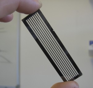
Once the sample DNA has been prepared adapters sequences are added to both ends of the fragment. The fragments are then attached to primer sequences on the flowcell (see figure 1). The result of this is that these single molecules are randomly scattered across the flow cell (A flowcell is simply a series of 8 glass channels each of which may contain a single (or multiplexed) sample). Sequencing by Synthesis could theoretically occur at this point, on the single molecule level. However it is unlikely that the fluorescence from a single molecule would provide enough signal to reliably sequence. In order to increase the signal “clusters” are grown from these single molecules using a technique called “bridge amplification”, this is a non-trivial, patent protect process. Once clusters have been grown the sample is loaded on to the device and sequencing can begin.

Figure 1: A GA1 Flowcell
Sequencing
The flowcell is loaded in to the device, the flowcell is manually focussed (an often problematic process!). Sequencing can now begin and occurs in a cyclic process, one cycle per read position. At the start of each cycle the flowcell is move under a peltier. The peltier heats the flowcell while the sequencing chemistry is performed. First, any “blockers” and labels are removed, leaving any previously incorporated bases attached. Labelled nucleotides are then washed over the flowcell. The nucleotides also contain a blocker, this prevents any additional nucleotides from incorporating and therefore ensures that in a single cycle only one base is added to each molecule.


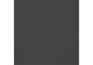
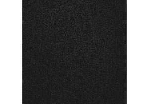
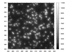
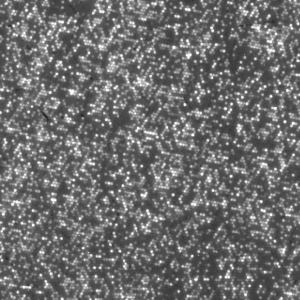
After the chemistry has been performed, imaging occurs. The flowcell is positioned under a CCD camera, and a laser is “bounced” off the bottom of the flowcell (so as to avoid it shining directly in to the CCD). The laser excites the fluorescent labels while the CCD camera takes a picture. Imaging is performed under 2 lasers and using 2 filters on the camera. This gives a total of 4 images per cycle, each of which reflects the luminescence, of one type of fluorophore/labelled nucleotide. The flowcell is imaged as a series of small, non-overlapping regions. In Solexa terminology these are called “tiles” (an example tile image is shown in figure 2. During a complete 36 cycle runs a single tile is composed of 4*36 images (4 channels times 36 cycles). On a GA1 these images are 1002x1004pixels, clusters are approximately 4 pixels in radius which corresponds to around 1micron.
The primary data analysis problem is therefore to segment and register each tile stack, and perform post image analysis corrections (basecalling) details of this can be found in the document entitled “The Solexa Pipeline” (I’ll have to upload this too sometime).
Error profile
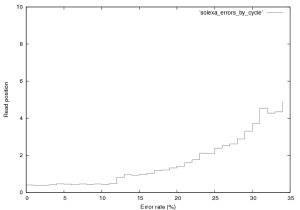
Figure 3 shows the distribution of errors in a Solexa run. 76,000 reads from a $\phi$X~174 control lane were aligned using a brute force alignment (which will find the best match with any number of errors). It therefore includes contamination, an analysis of which is provided elsewhere (contact new at sgenomics dot org for more information). Quality scores were not used in alignment. It should also be noted that this is the error rate for the PF fraction of the data, this is all a user normally sees. In Solexa sequencing errors tend to follow this basic trend, increasing slowly with read length upto around 5% in the final cycle. Early cycle errors tend to be around 0.3 to 0.5% and we believe are mostly caused by contamination. Errors increase with cycle for two basic reasons, the first is single loss. As cycle progresses the fraction of molecules that no longer produce signal increases (through photobleaching, chemical, or physical effects). Secondly the number of molecule that are “out of phase” with the current cycle increases and can no longer be corrected for by the primary data analysis software. Phasing is caused by the non-incorporation of a labelled base or non-blocking of a labelled base (and therefore the incorporation of too many bases), this manifests itself as signal leakage between cycles. The jump in error rate at cycle 12 is caused by purity filtering (the minimal purity over the first 12 bases is used).

Figure 3: Error rate by cycle in a Solexa $\\phi$X~174 control lane (not a great run, GA1), this plot was created from the first 76,000 reads in this provided dataset.
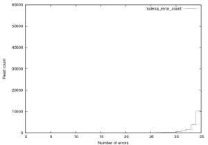
Figure 4 shows the distribution of errors, 35 being fully correct. As expect errors are relatively evenly distributed thoughout reads. If you look at the entire dataset (not just PF) a similar trend is seen, errors start at a much higher level and the error rate in the total dataset is around 6%.

Figure 4: Distribution of errors a Solexa $\\phi$X~174 control lane (not a great run, GA1), this plot was created from the first 76,000 reads in this provided dataset.
Focusing
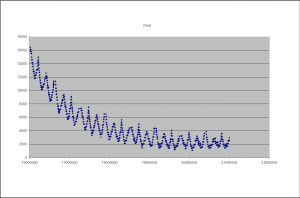
During imaging the camera refocuses between tiles, this results in a change in the Z-height on the camera (as it moves up and down to focus). Guoying Qi at the Sanger institute has made the following plots of the Z-height as the images progresses. Figure 5 shows the Z-height for a single cycle. There are two interesting artifacts in these plots, which tell us something about the underlying technology. The first is the sawtooth pattern in Z-height. The peaks of these occurs at the extreme ends on the lanes (channels on the flowcells). In this case the Z-height is slowly decreasing as the end of the lane approaches, it then abruptly begins to increase as the camera walks back down the flowcell (images are taken in a zig-zag pattern). This indicates that the flowcell is not perfectly flat in its mounting and is sloped along its Y-axis.

Figure 5: The Z-Height for cycle 2 across all tiles/lanes
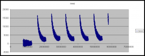
The second artifact is the gradual decay in Z-height as the cycle progresses. Our current theory is that this is a temperature dependent effect, the ambient temperature of the in higher at the beginning of the cycle, due to the heat produced by the peltier while base incorporation is performed. This causes the flowcell to warp slightly altering the focusing. As the ambient temperature is approached the flowcells original shape is restored and the Z-height decreases. This is perhaps backed up by the fact that the first cycle often does now show this decay in Z-height (see figure 6).

Figure 6: The Z-Height for all tiles/lanes across the first six cycles
454
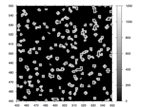
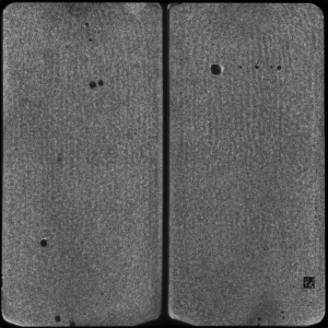
I know very little about 454 sequencers, other than that the primary data analysis is the most closed of the 3 platforms. Images are stored in a proprietary “pif” format, for which no documentation is available (update: if I remmember correctly pifs are actually tiff files with a few bytes on the front).
454 Sequencers produce reads of appoximately 100~bp, however the throughput is not as high as Illumina or ABI’s and the cost per base is higher (so I’m told). They also have significant problems with “homopolymer runs”, that is runs of the same base. The 454 technology produces an intensity trace where a higher peak represents a longer run of the same base, this causes some ambiguity.
Update: So, I really don’t know that much about the underlying technology of 454 sequencers, and I’ve never worked with the data but essentially like Ion torrent machines and unlike Solexa sequencers the don’t have dye terminators. This is what causes the homopolymer problems, as more than one base can incorporate in a single “flow”. The dye terminator technology is patented, and I assume difficult to license/get around. If you could use the dye terminator technology from Ilm on an Ion torrent machine, that would probably improve things quite a lot (as always this is random speculation and guessing).

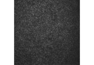
Figure 7: A 454 Tile image

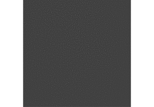
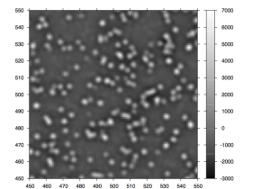
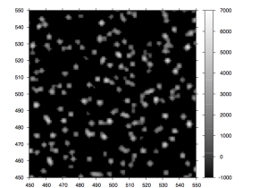
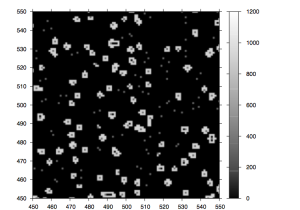
Figure 8: Magnified region of a 454 tile image.
Solid
The ABI SOLiD is a next-gen, high-throughput, sequencing by ligation, DNA sequencer. The ABI SOLiD sequencing system is significantly different from both traditional Sanger sequencing and other high throughput DNA sequencers. In terms of informatics this is largely apparent by the novel 2 base encoding system employed by the device.
The technique first attaches prepared DNA samples to beads. Each bead contains PCR amplified copies of a single molecule. Beads are then attached to the surface of a flowcell. The sequencing then operates in a cyclic process though the ligation of successive “probe” sequences to the beads. Each probe is ligated, read (via it’s fluorescence) and then removed. This is further complicated by the use of five different primers to offset probes and allow the reads to completely cover the target, however this is not a significant issue from an informatics perspective.
Each ligation probe is composed of 3 degenerated bases (all possible 3~bp sequences synthesised combinatorially (CHECK)) followed by a 2~bp read sequence, and then 3 fluorescently labelled universal bases. Degenerate bases are used to provide a discrimination advantage [drmanac02] during hybridisation. An example probe might be: 3′ NNNATZZZ 5′.
Ideally this probe would hybridise and be ligated against 5′ NNNTANNN 3′ in the sample. The probe is designed such that it fluoresces in a given channel. Table 1 shows the channel (colour) that is emitted by a given probe.
Table 1: ABI Solid base to colour chart. Different dyes are represented as numbers. In ABI documentation these are usually denoted by the following colours: 0. Blue 1. Green 2. Orange 3. Red. and represent these dyes: 0. 6-FAM 1. CY3 2. Texas Red 3. CY5
Basecalling
Table 2: From table 1 we can determine the colour to sequencing mapping shown.
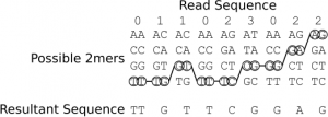
As you can see the sequencer adopts a novel 2 base encoding strategy. That is a single 2bp combination does not emit a unique signal, but one that is shared amongst 3 others. In order order disambiguate these signals and obtain base calls you therefore need to trace a path from signal symbol to signal symbol (colour to colour), and in order to do this unambiguously you need to know the first base in the sequence. When sequencing this is known as the first base is part of the primer sequence. Table 2 shows the colour to base mapping which can be inferred from table 1. An example disambiguation of the read sequence 011023022 is shown in figure 9.

Figure 9: An example showing the conversion of the colour sequence 011023022 and a known starting base (T) in to a base sequence: TTGTTCGGAG
SNP Calling
SNP calling is the process of identifying single nucleotide changes in a genome with respect to a reference sequence. Traditionally this is performed by aligned reads against a reference and noting differences between the alignment and reference. It is usual to require a large number of reads covering a given SNP in order to confirm the call.
This method can also be used with the ABI SOLiD. That is to say, a colour space sequence is translated in to a base pair sequence, which is then aligned to the genome in order to identify SNPs. However there maybe certain advantages to aligning in colour space directly in this case the reference sequence is translated in to colour space. Colour space reads are aligned to the colour space reference, these regions are then translated back to sequence space and SNPs called. As we shall see this has a number of advantages in the identification of miscalls.
When errors occur
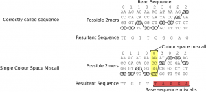
Miscalled, inserted or deleted colours manifest themselves similarly in terms of base space, that is they significantly alter the base calls of all remaining bases in the read, this is because subsequent base calls are dependent on previous base calls which causes the error from one call to propagate though all subsequent bases, figure 10 illustrates this effect.

Figure 10: The effect of a single colour space miscall on base pair sequence
Advantages of miscall errors for SNP calling
One of the marketed features of the ABI SOLiD is that this error propagation has an advantage for SNP calling, and is their main reason for employing colour space alignments. The reasoning is as follows: “if you align in colour space to a position that contains a single mismatch then you have a high degree of confidence that this read came from this location, however because the read and reference are vastly different in terms of sequence this is likely to be a miscall”. Let’s try to quantify this.
* Reads align to a unique location, the number of allowable mismatches will need to be tuned such that this is the case, or significant problems will occur.
* If there is a single colour mismatch at position $t$ of a read of length $l$ then this SNP is really a miscall or this and subsequent bases are mutated to one of $4^{l-t}$ sequences. Therefore the probability of this being a true call at the position in the sequence is $c = \frac{1}{4^{l-t}-1}$ given that all alternate sequences are equally likely (some may contain more mismatches than others but we take this as a close approximation). The probabilities for a 25~bp read are shown in table~\ref{miscall-probabilities}. If $d$ (the device miscall probability) is greater than $c$ (probability of mismatches in the remainder of the read) then it more likely that this base has been miscalled.
Table 3: Probabilities of a single colour space miscall being a true base pair sequence in a 25~bp read: %octave: for t= 1:24;l=25; c = (1/(4^(l – t) – 1));printf(“%e\n”,c); end for
If the mismatch occurs in the last base then we have no other information to base the probability that this is a miscall on, it’s likelihood is therefore $d$ (probability of a miscall based on device characteristics). These probabilities however are based on the notion that this data came from this location on the reference. We must therefore tune the minimal number of allowable alignment matches such that it is unlikely that is read came from an alternate location. The number of times we would expect any given 25~bp read with $m$ or fewer mismatches appear in a randomly distributed human genome sized sequence ($3.2\times10^9$~bp) is shown in table~\ref{human-mismatch-alignment}, the method used to generate this is described in the appendix. Even though it has previously been shown that substring in the human genome are not randomly distributed [whiteford05] [whiteford08] we can only expect these values to degenerate as order increases and they therefore provide an acceptable upper bound. From this table we can see that with 25~bp reads, we can only allow up to 3 mismatches. For 35~bp reads this increases to 8~mismatches and at 50~bp we have reached 16~mismatches. This is confirmed in practice where 25~bp reads with greater than 3 mismatches align poorly or to multiple locations (NOTE: multiple locations true?). It should also be noted that mismatches are not just due to miscalls but also true SNPs which as we shall see later cause 2 mismatches, with 25~bp reads we can therefore expect to identify 1 SNP and allow one mismatch before the read is no longer alignable.
Given a device miscall rate $d$, the probability of a read of length $n$ containing $m$ or more miscalls is:
\begin{equation}
s = \sum\limits_{k=1}^{m}\frac{n!}{k!(n-k)!}(d^k(1-d)^{n-k})
\end{equation}
and therefore can expect to discard $100\times s$ percent of reads, this is tabulated in table~\ref{discarded} for varying error rate and read length taking the maximal read lengths identified in~\ref{human-mismatch-alignment}.
\begin{center}
\begin{table}[h]
\begin{center}
{\footnotesize
\begin{tabular}{ | r | c | c | c |}
%octave: d=0.1; n=50; m=50;s=0; for k=17:m; s=s+sum((factorial(n)/((factorial(k)*factorial(n-k))))*d^k*(1-d)^(n-k)); endfor; printf(“%d %f\n”,k,s);
\hline
Error rate & 25~bp read, $\geq$4~mismatches & 35~bp read, $\geq$9~mismatches & 50~bp read, $\geq$17~mismatches \\
\hline
0.005 & 0.0007\% & 0.0\% & 0.0\% \\
0.01 & 0.0107\% & 0.0\% & 0.0\% \\
0.02 & 0.1446\% & 0.0\% & 0.0\% \\
0.03 & 0.6186\% & 0.0001\% & 0.0\% \\
0.04 & 1.6522\% & 00.0007\% & 0.0\% \\
0.05 & 3.4091\% & 00.0042\% & 0.0\% \\
0.06 & 5.9757\% & 00.0170\% & 0.0\% \\
0.07 & 9.3612\% & 00.0533\% & 0.0\% \\
0.08 & 13.5092\% & 00.1388\% & 0.0\% \\
0.09 & 18.3146\% & 00.3130\% & 0.0001\% \\
0.1 & 23.6409\% & 00.6304\% & 0.0004\% \\
0.2 & 76.6007\% & 25.4988\% & 1.4442\% \\
\hline
\end{tabular}
}
\caption{Percentage of reads which will be unalignable, or misaligned due to high numbers of errors for varying error rate and read length.}
\label{discarded}
\end{center}
\end{table}
\end{center}
\begin{center}
\begin{table}[h]
\begin{center}
{\footnotesize
\begin{tabular}{ | r | c | c | c |}
\hline
%octave: l=3200000000; m=0; for k=1:25; n= 25; g = (3^k)*(factorial(n)/(factorial(k)*factorial(n-k))); m=m+g; e=(m/(4^n))*(l-n+1); f=l/e; printf(“%d %d %d %e %e\n”,k,g,m,e,f); endfor
Mismatches in alignment $m$ & Alignments ($n$ = 25~bp) & Alignments ($n$ = 35~bp) & Alignments ($n$ = 50~bp) \\
1 & $2.131628\times10^{-4}$ & $2.846031\times10^{-10}$ & $3.786532\times10^{-19}$ \\
2 & $7.887024\times10^{-3}$ & $1.479936\times10^{-8}$ & $2.820967\times10^{-17}$ \\
3 & $1.843858\times10^{-1}$ & $4.937863\times10^{-7}$ & $1.364098\times10^{-15}$ \\
4 & $3.096616$ & $1.198947\times10^{-5}$ & $4.845417\times10^{-14}$ \\
5 & $3.979072\times10^{1}$ & $2.258093\times10^{-4}$ & $1.348140\times10^{-12}$ \\
6 & $4.067318\times10^{2}$ & $3.433106\times10^{-3}$ & $3.059108\times10^{-11}$ \\
7 & $3.394680\times10^{3}$ & $4.329522\times10^{-2}$ & $5.820293\times10^{-10}$ \\
8 & $2.356333\times10^{4}$ & $4.618474\times10^{-1}$ & $9.473970\times10^{-9}$ \\
9 & $1.378524\times10^{5}$ & $4.228817$ & $1.339611\times10^{-7}$ \\
10 & $6.864397\times10^{5}$ & $3.361118\times10^{1}$ & $1.665153\times10^{-6}$ \\
11 & $2.930661\times10^{6}$ & $2.339455\times10^{2}$ & $1.836907\times10^{-5}$ \\
12 & $1.078543\times10^{7}$ & $1.435951\times10^{3}$ & $1.812322\times10^{-4}$ \\
13 & $3.434975\times10^{7}$ & $7.815829\times10^{3}$ & $1.609417\times10^{-3}$ \\
14 & $9.494372\times10^{7}$ & $3.789239\times10^{4}$ & $1.293288\times10^{-2}$ \\
15 & $2.282504\times10^{8}$ & $1.642140\times10^{5}$ & $9.446183\times10^{-2}$ \\
16 & $4.782005\times10^{8}$ & $6.379199\times10^{5}$ & $6.294956\times10^{-1}$ \\
17 & $8.751801\times10^{8}$ & $2.226228\times10^{6}$ & $3.839698$ \\
18 & $1.404486\times10^{9}$ & $6.991152\times10^{6}$ & $2.149581\times10^{1}$ \\
19 & $1.989509\times10^{9}$ & $1.978121\times10^{7}$ & $1.107056\times10^{2}$ \\
20 & $2.516029\times10^{9}$ & $5.047735\times10^{7}$ & $5.255314\times10^{2}$ \\
21 & $2.892115\times10^{9}$ & $1.162548\times10^{8}$ & $2.303356\times10^{3}$ \\
22 & $3.097253\times10^{9}$ & $2.418299\times10^{8}$ & $9.333844\times10^{3}$ \\
23 & $3.177524\times10^{9}$ & $4.547617\times10^{8}$ & $3.501041\times10^{4}$ \\
24 & $3.197592\times10^{9}$ & $7.741593\times10^{8}$ & $1.216688\times10^{5}$ \\
25 & $3.200000\times10^{9}$ & $1.195764\times10^{9}$ & $3.920430\times10^{5}$ \\
26 & NA & $1.682231\times10^{9}$ & $1.171969\times10^{6}$ \\
27 & NA & $2.168698\times10^{9}$ & $3.251770\times10^{6}$ \\
28 & NA & $2.585670\times10^{9}$ & $8.376996\times10^{6}$ \\
29 & NA & $2.887615\times10^{9}$ & $2.004130\times10^{7}$ \\
30 & NA & $3.068782\times10^{9}$ & $4.453635\times10^{7}$ \\
31 & NA & $3.156444\times10^{9}$ & $9.194611\times10^{7}$ \\
32 & NA & $3.189317\times10^{9}$ & $1.763948\times10^{8}$ \\
33 & NA & $3.198282\times10^{9}$ & $3.145834\times10^{8}$ \\
34 & NA & $3.199864\times10^{9}$ & $5.218665\times10^{8}$ \\
35 & NA & $3.200000\times10^{9}$ & $8.061403\times10^{8}$ \\
36 & NA & NA & $1.161483\times10^{9}$ \\
37 & NA & NA & $1.564844\times10^{9}$ \\
38 & NA & NA & $1.978821\times10^{9}$ \\
39 & NA & NA & $2.360953\times10^{9}$ \\
40 & NA & NA & $2.676211\times10^{9}$ \\
41 & NA & NA & $2.906889\times10^{9}$ \\
42 & NA & NA & $3.055181\times10^{9}$ \\
43 & NA & NA & $3.137949\times10^{9}$ \\
44 & NA & NA & $3.177452\times10^{9}$ \\
45 & NA & NA & $3.193253\times10^{9}$ \\
46 & NA & NA & $3.198406\times10^{9}$ \\
47 & NA & NA & $3.199721\times10^{9}$ \\
48 & NA & NA & $3.199968\times10^{9}$ \\
49 & NA & NA & $3.199998\times10^{9}$ \\
50 & NA & NA & $3.200000\times10^{9}$ \\
\hline
\end{tabular}
}
\caption{Expected number of alignments with $m$ or fewer mismatches for reads of length $n$ against a genome of $3.2\times10^9$~bp. Values less than one mean that in a randomly distributed sequence of this size we would expect reads with $m$ mismatches to be unique.}
\label{human-mismatch-alignment}
\end{center}
\end{table}
\end{center}
So far we have determined how many miscalls will cause our reads is misalign, we have also shown that given a good alignment the probability of a colour mismatch toward the end of a read being caused by a miscall decreases toward the end of a read. We now address the question of true SNPs, how they effect colour space sequence and given a particular colour space miscall rate what the SNP miscall rate is.
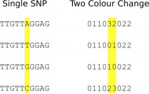
As shown in table~\ref{miscall-probabilities} in most read positions the probability of a single colour change being due to a true sequence polymorphism is low. In current protocols therefore all single colour changes are discarded. A true independent SNP will cause two consecutive changes in colour space to one of 3 other two colour combinations, as shown in figure 11. It should also be noted that a true SNP call can not be registered incorrectly by a single miscall, two colour changes are required to change a valid SNP in to an alternate valid single SNP colour sequence. Given this the question is therefore at a given device miscall rate what therefore is the probability of two consecutive miscalls causing a valid two colour change?

Figure 11: An example showing the two colour changes that are caused by single, real SNPs
The probability of two consecutive miscalls is $d^2$ (where $d$ is the device error rate), out of the $4^2$ colour combinations 3 would be interpreted as valid SNP calls the final single SNP misscall probability is therefore $f = \frac{3d^2}{4^2}$.
Theoretical Conclusions
We have shown that an ABI device with a miscall rate of $d$ has a SNP call rate of $\frac{3d^2}{3^2}$.
Current ABI devices have a miscall rate of 0.1 (based on the Q scores in the Yoruba dataset, however these are not evenly distributed across reads so, this may be unfair). They therefore have a SNP calling error rate of 0.0033 (0.33\%, approximately Q25) which is comparable with that obtainable from Solexa devices. We have also determined the number of mismatches that may be tolerated before alignments repeat, it is crucial to the error correction process that the alignment maps against the correct position on the reference. For a 25~bp read against a human genome size sequence of random distribution we have shown that a maximum of 3 mismatches can be tolerated, effectively 1 true SNP and 1 error and that at an error rate of 0.1, 23\% of reads would have 4 or more errors, and would therefore not align or misalign. Reducing the device miscall rate to 0.05 would result in a final SNP call error rate of approximately Q31. Increasing the read length from 25~bp to 35 or more would would decrease the probability of misalignment significantly.
In this document we have only discussed the use of ABI sequence data for SNP calling. DNA sequencer will typically also be used for \emph{de novo} assembly of read sequences. The ABI SOLiD will not be able to take advantage of it’s ability to correct against a reference here and we will be left with the raw error rate when overlapping reads.
Distribution of Errors in the E.Coli Dataset
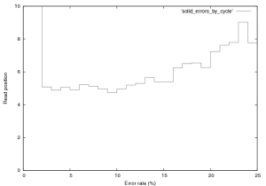
76,000 reads from the SOLiD v.2 E.Coli dataset provided by ABI were aligned. Only the first end read was used, which in this dataset was 25~bp. I used a bruteforce aligner (which accepts any number of errors) to align this data, the aligner does not factor quality scores in to its alignment. The reference sequence was translated in to colour space, and the reads aligned. The purpose of this analysis is to get a handle on the single colour change error rate, and the distrubtion of errors in the reads. Figure 12 show the error rate by cycle. Cycles one and two have predictably high error rates, the first is not a colour space symbol (a “T”) and therefore results in a 100% error rate. The second can not be interperated correctly in colour space (as it partly covers the adapter and the real sequence), its alignment is therefore almost random and therefore has a high error rate.
Interperation of the error rates on the remaining cycles is difficult. I expect to see a more significant bias due to the order in which the ligation probes are added, when compared to the ligation order some correlation does appear to exist but it is not hugely significant. A trend toward increase error which increasing cycle does exist, as does a significant peak in errors on the penultimate base (Erin: you told me why, but I can’t remember).
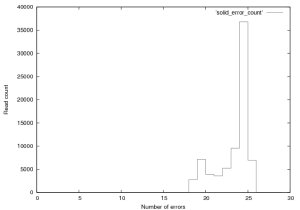
Figure 13 shows the distribution of errors in these reads. 2771reads had 18 errors, while only 13 had 17 errors (these could be alignments that overlapped with “N”s which were not converted in to colour space sequence. Such a large drop is unlikely and suggests that the dataset may have been filtered to remove poorly aligning reads.

Figure 12: Error rate by cycle in SOLiD v.2 E.Coli Dataset, this plot was created from the first 76,000 reads in this provided dataset.

Figure 13: Distribution of errors per read in SOLiD v.2 E.Coli Dataset, this plot was created from the first 76,000 reads in this provided dataset. Reads of score 24 or 25 should be considered “fully correct”.
Appendix
Enumerating Mismatched Alignments
In order to enumerate the number of possible mismatches in a sequence of length $n$ we first determine the number of possible mismatch positions. This is a simple exercise in combinatorics but is perhaps best illustrated with an example. If we have a sequence of length 5 ($n = 5$) then mismatches can occur at positions $1, 2, 3, 4$ or $5$. We wish to know the number of possible sequences with 3 mismatches ($k = 3$). This is simply the binomial coefficient [knuth73a-binomial] (colloquially, the number of ways to pick $k$ objects out of $n$ options):
\begin{equation}\frac{n!}{k!(n-k)!}\end{equation}If we are interested in the number of strings of length $n$ with $m$ or less mismatches we therefore have:
\begin{equation}
g_{n,m} = \sum\limits_{k=1}^{m}{3^k\times\frac{n!}{k!(n-k)!}}\end{equation}
As each position of each mismatch can be one of 3 alternate bases. If we would like to know the number of times we would expect to see a match within $m$ mismatches of a string of length $n$ against a randomly distributed target string of length $l$ we have:
\begin{equation}e = \frac{g_{n,m}}{4^n}\times(l-n+1)\end{equation}
As $g_{n,m}/4^n$ is the number of times we would expect to see this sequence in any given alignment position and $(l-n+1)$ is the number of alignment positions in the target sequence.
[drmanac02]: Sequencing by Hybridization (SBH): Advantages, Achievements, and Opportunities, R.Drmanac et al., abeb, 77, 2002, July 75
[sanger77]: DNA Sequencing with chain-terminating inhibitors, F Sanger et al., Proceeding of the National Academy of Sciences U.S.A., 74, 1977, 5463-5467
[whiteford05]: An analysis of the feasibility of short read sequencing, N Whiteford et al., bar, 33, 19, e171-, 2005
[whiteford08]: Visualizing the Repeat Structure of Genomic Sequences, N Whiteford et al., Complex Systems, 17, 4, 2008
[knuth73a-binomial]: The Art of Computer Programming (Volume I): Fundamental Algorithms, D. E. Knuth, 51–73, 1973
