Z1 Coulter Particle Counter Teardown

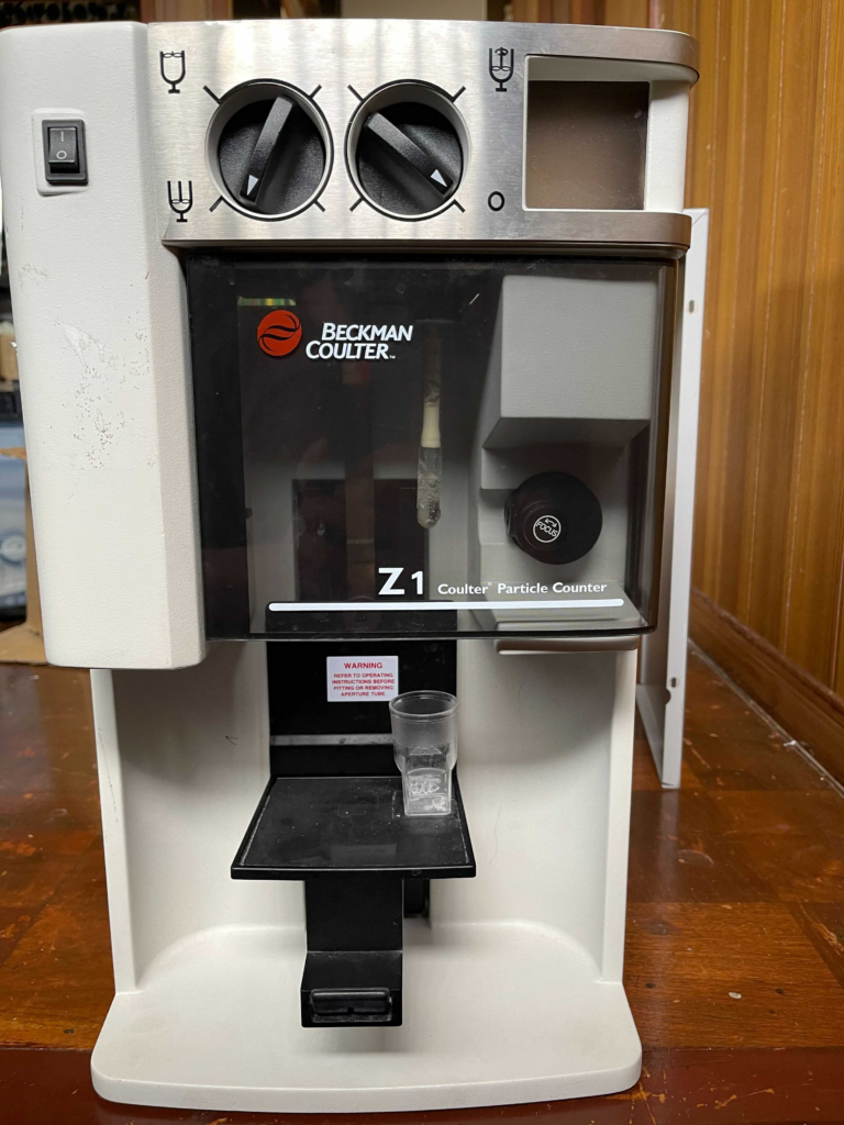
I picked up a Beckman Coulter Z1 particle counter on eBay. I suspect it was non-functional. The control pad was missing and the rear case only had one screw. But this was fine for me as I was mostly interested in pulling it apart.

I’ll cover the aperture and fluidics first here. A dump of the pictures of the rest of the unit can be found at the end of this post.

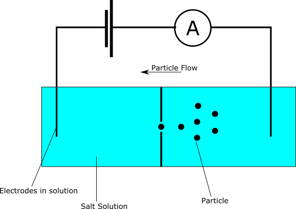
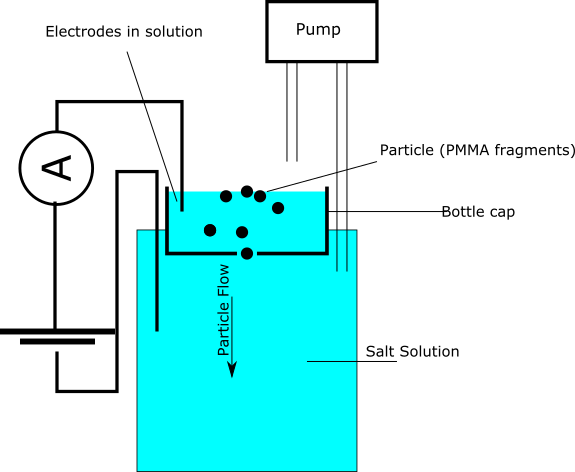
Coulter counters are used to measure particle sizes. For example, to gain red and white blood cell counts. They do this by suspending particles in a conductive (salt) solution. This fluid is then driven through a aperture. A bias voltage is passed over the aperture and the current flowing through the aperture is measured. The fluid is driven through the aperture under pressure. As particles pass through the aperture they block the current flow, and can therefore be detected/counted.

The principle is discussed in a previous blog post.

Aperture

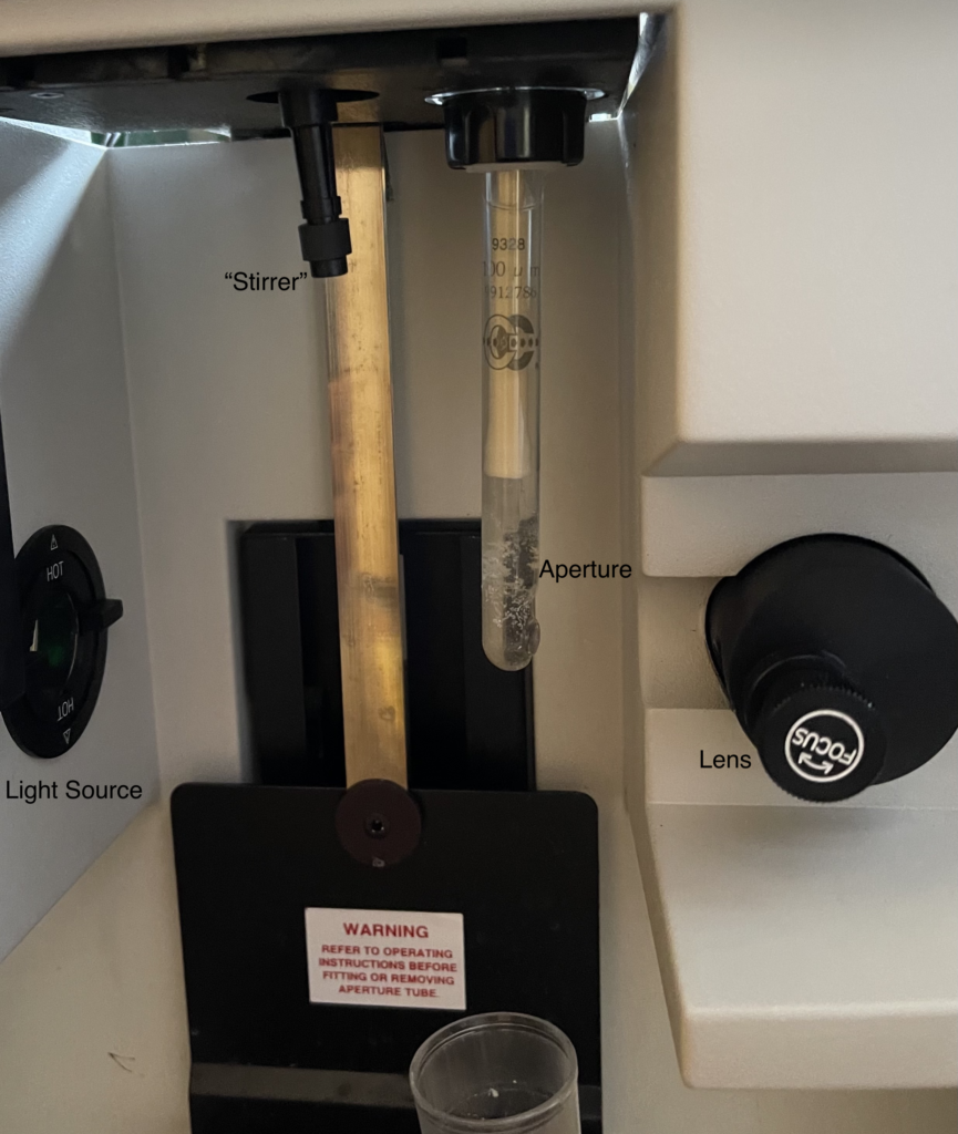
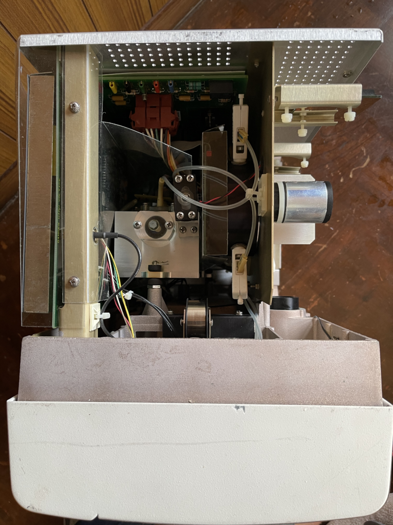
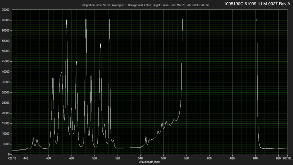
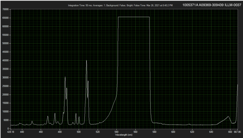
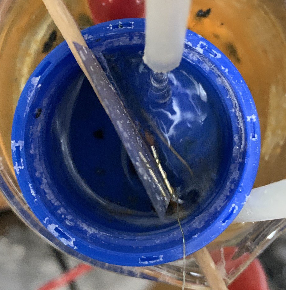
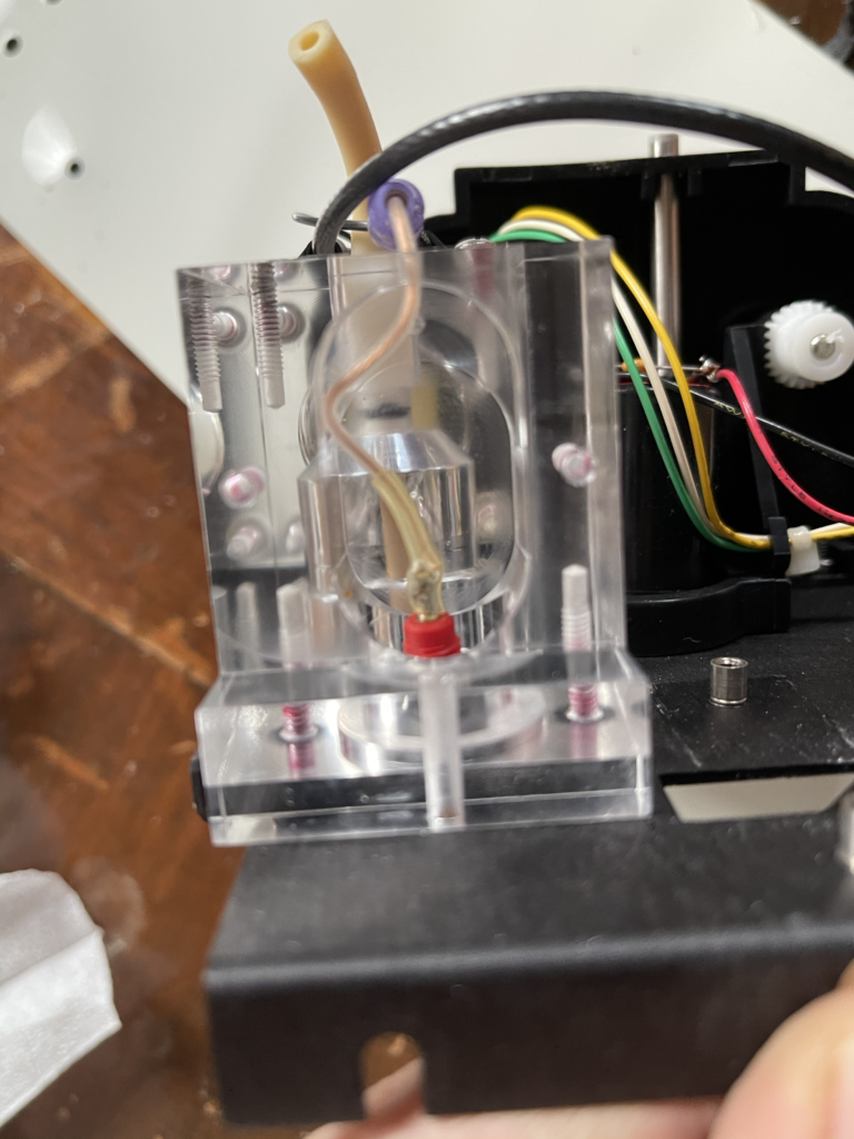
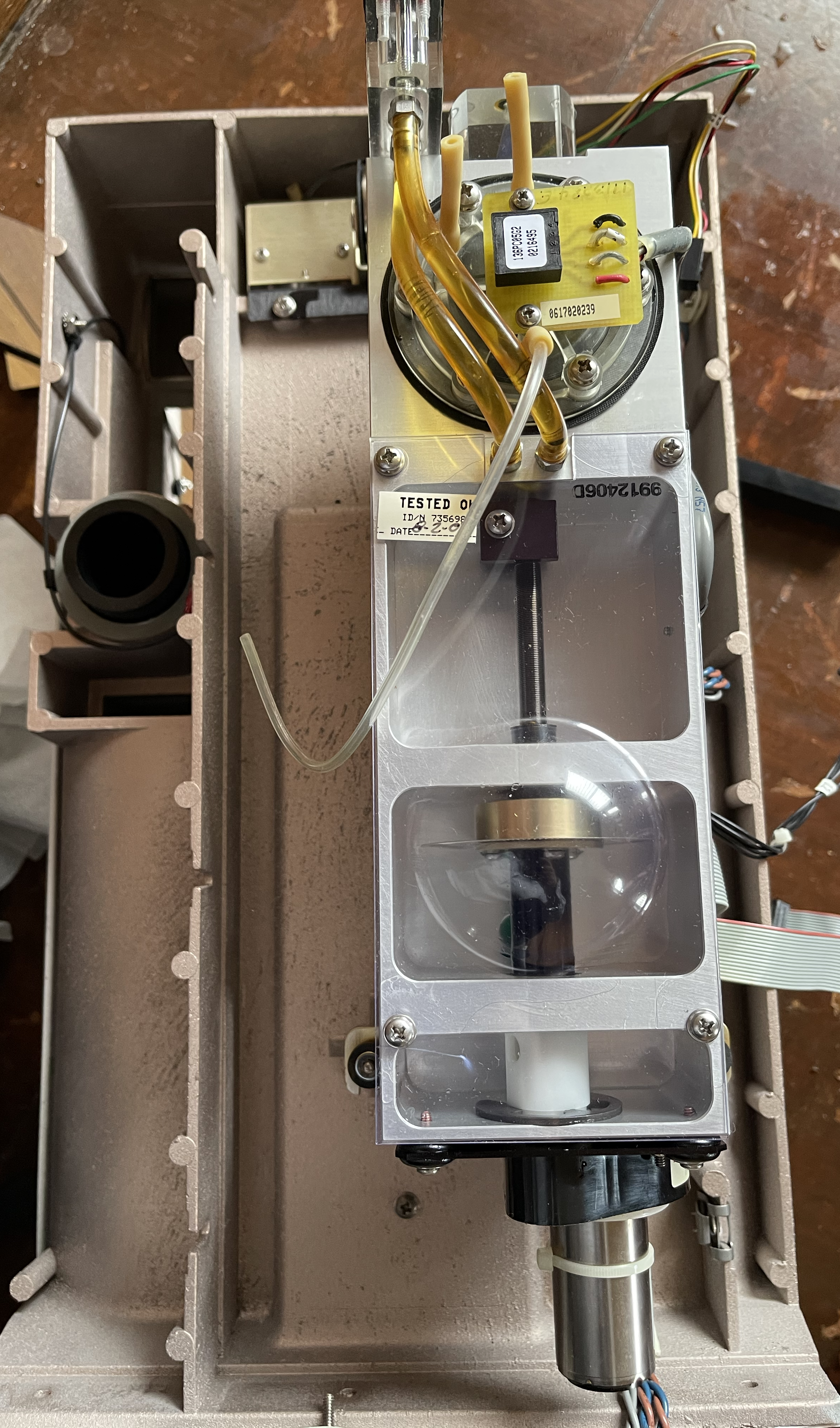
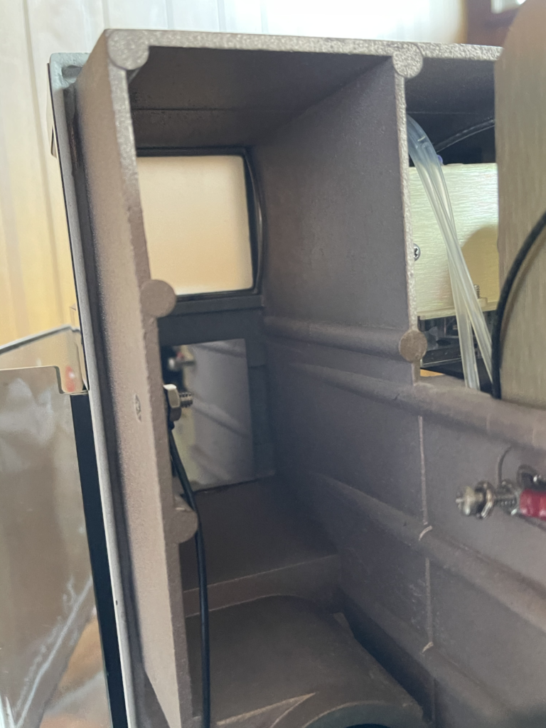
The aperture “rod” screws into the unit. There’s a light source (Mercury lamp I think) which can be used to illuminate the aperture. This is focused through the lens on the right and projected on to a screen at the top of the unit. The system is purely optical, there’s no detection electronics. It’s unclear to me how clear the alignment of the aperture is… or what the exact purpose of optically monitoring the aperture is.

There’s a stirrer attachment to the left of the aperture rod. From the rest of the system I suspect this also makes electrical contact with the fluid.

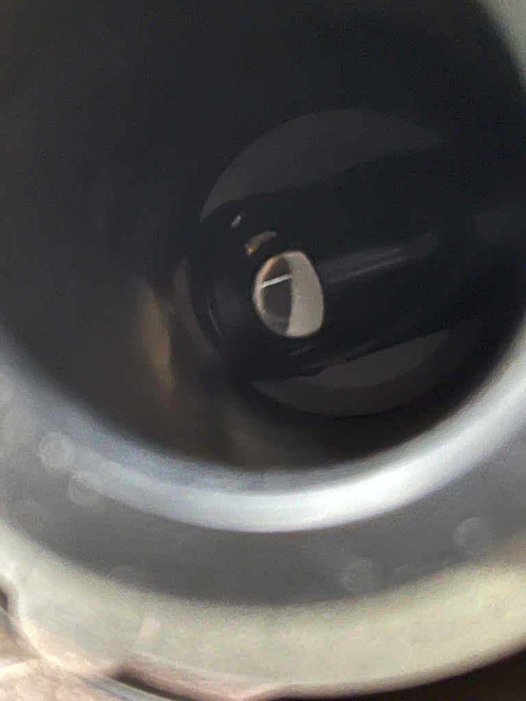
The aperture rod itself is a glass tube:

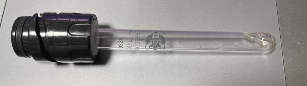
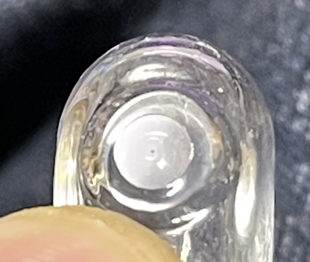
At the end of the tube is a flat disc with a small aperture in it. It’s not clear to me if this is a polished part of the glass or a disc embedded in it:

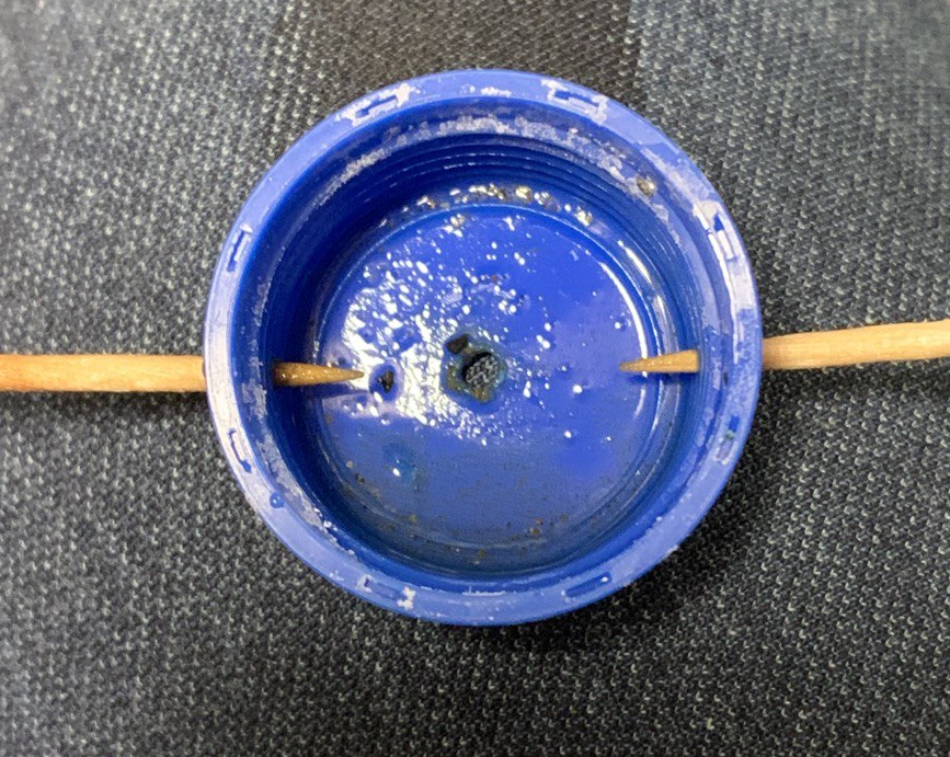
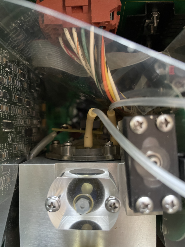
If you pull apart the instrument, you’ll find the aperture attaches to a small fluidic block:

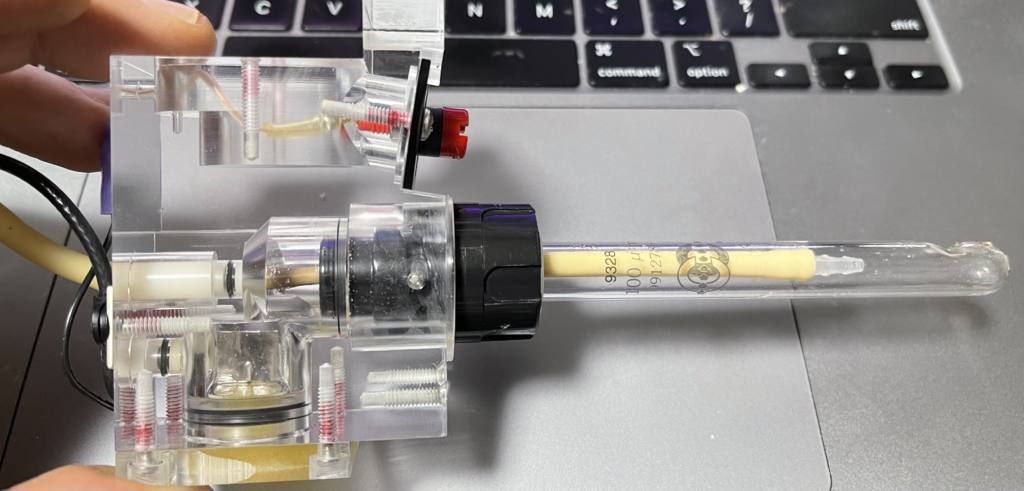
The coax cable on the left makes contact with the foil sheet on the bottom (with is in the interior tube fluid path) of the unit and the red connector on the top of the unit. Somehow this top red connector must make contact with the sample. I assume via the stirrer…

There are two fluidic connectors at the top of the block. I imagine the instrument can pre-fill the tube via one of these.

Fluidics

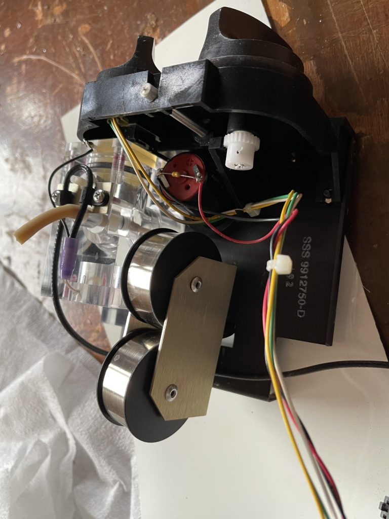
The bulk of the instrument is composed of two fluidic components. A selector valve, and a metering pump.

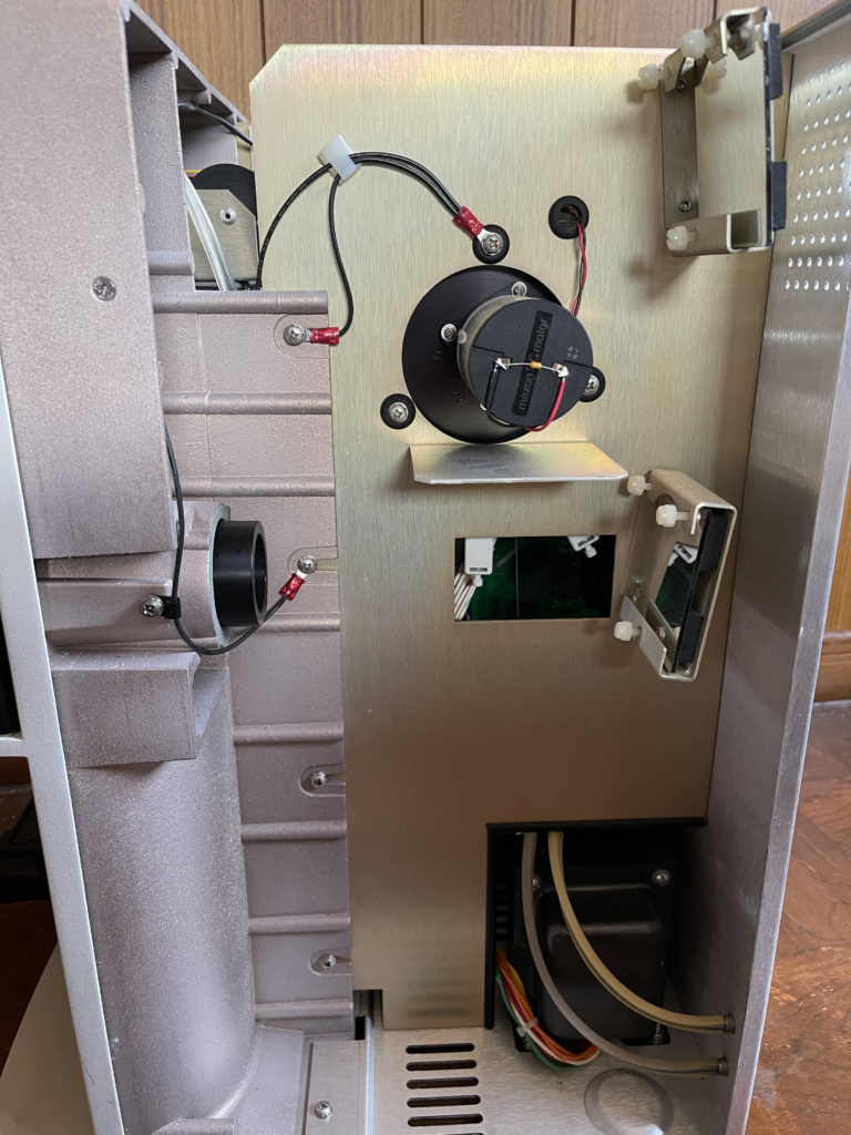
The metering pump, labeled “Metering Module”. Is a rather attractive piece of engineering:

Pump “front”
Pump “rear”

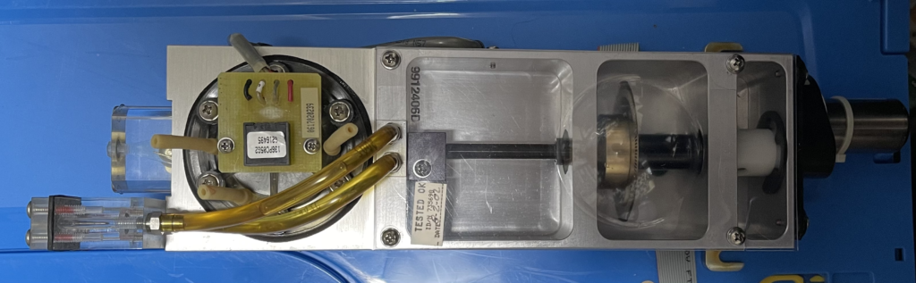
It appears to essentially be an oil filled diaphragm pump. On the “front” of the unit above you can see a Maxon DC motor to the right. This drives a rod with an encoder wheel on it. The rod feeds through into the oil chamber.

By pushing the rod into the chamber the oil push pressure on a membrane which can be used to move fluid around…

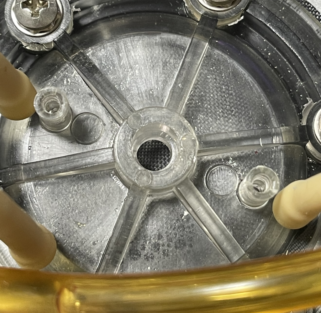
This membrane makes contact with the fluid on the other side of the pump (“front” above”):

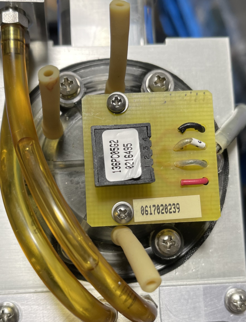
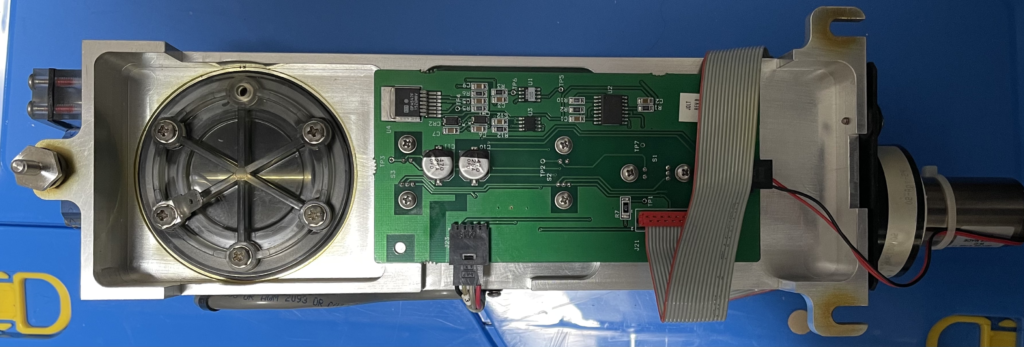
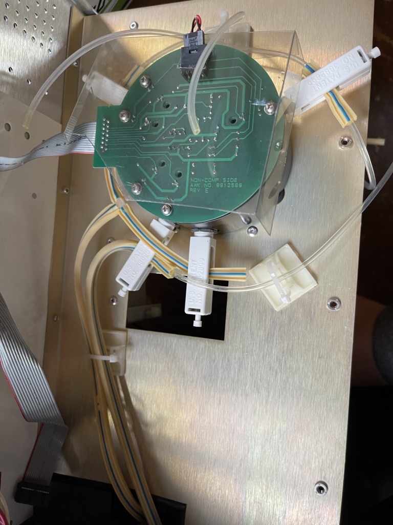
The three fluidic connectors/tubes above all make contact with the main chamber containing the diaphragm. The component on the PCB above also makes contact with the chamber, and I would guess is almost certainly a pressure sensor:

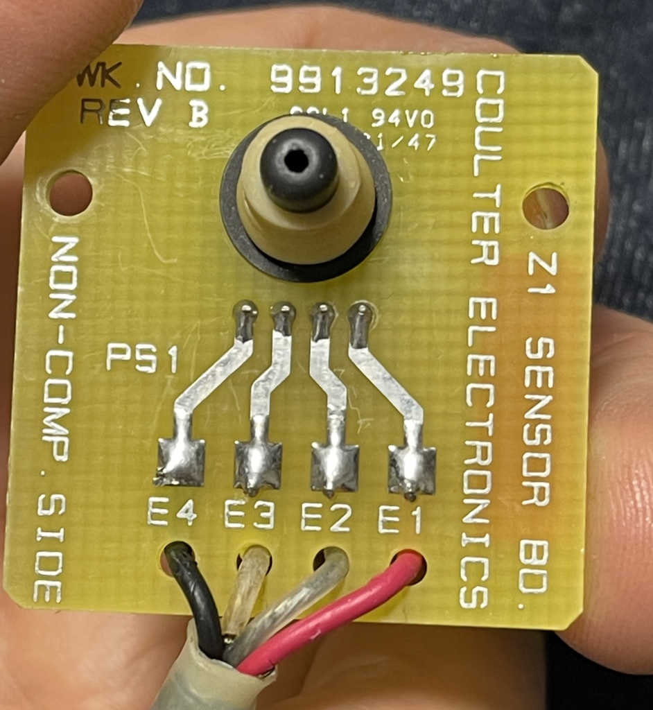
With the pressure sensor removed you can just see the membrane:

As it goes, this is all fine. But in order to move fluid around, the diaphragm pump needs a valve to open and close the inputs/outputs. In a regular diaphragm pump these are usually mechanical valves:

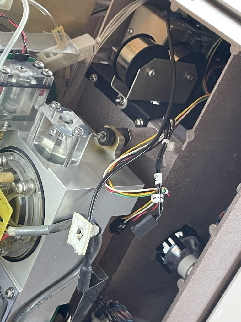
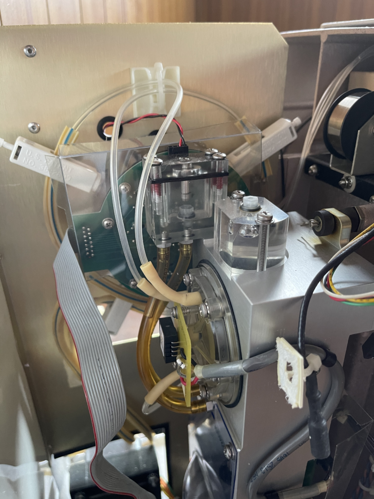
But in order to allow the pump to switch between different inlets/outputs the Z1 uses a motor driven selector valve:

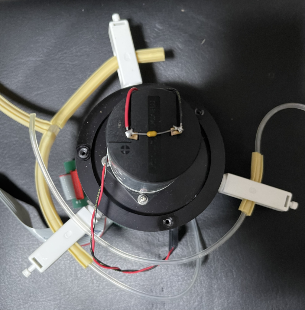
This is a very simple mechanical system. The white valves just clamp tubes shut under pressure:

Inside the unit is a wheel which is rotate by the motor to put pressure on the values:

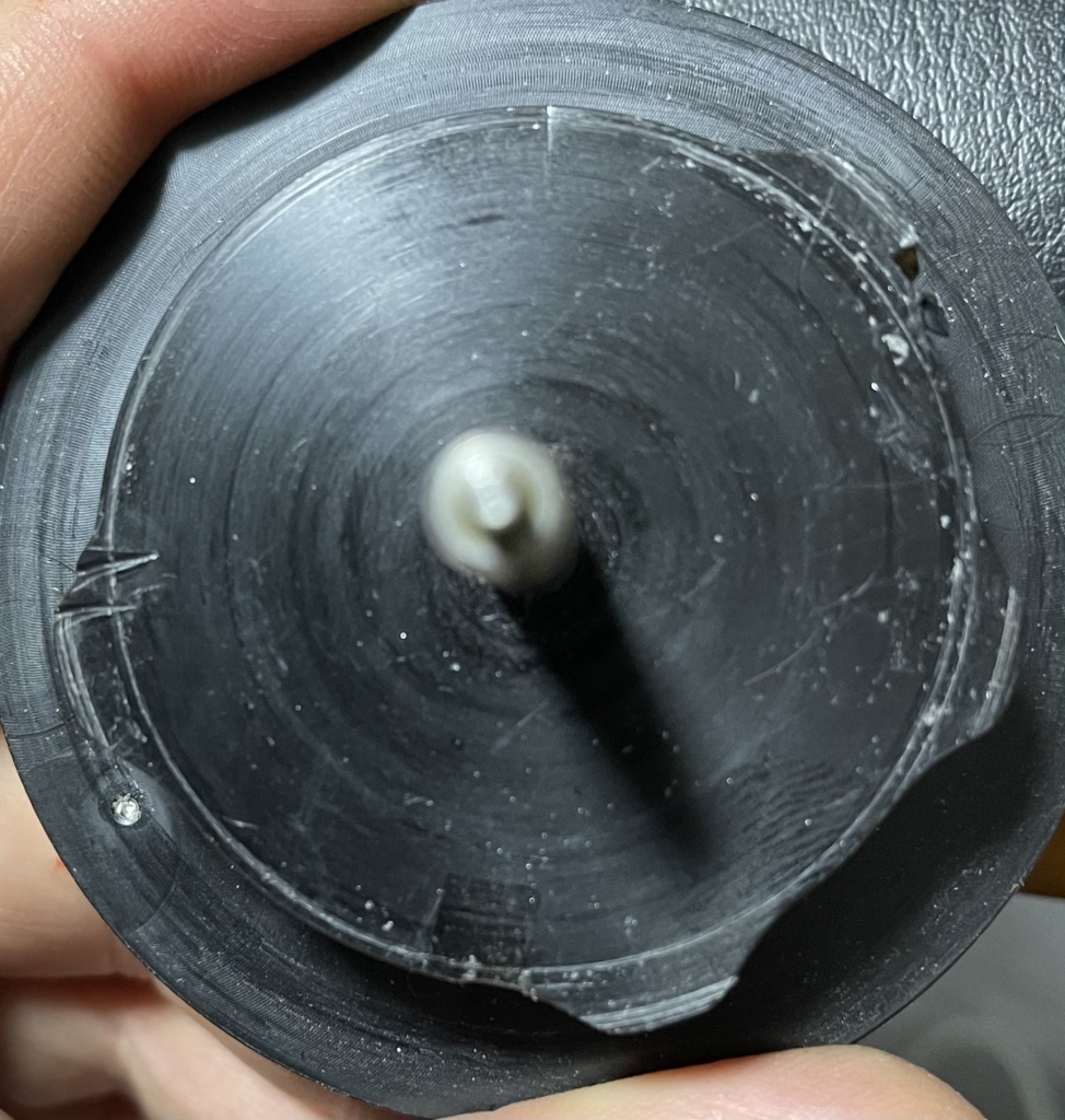
For the most part this wheel seems to clamp down on one valve at a time. So I would imagine this can be used to first fill the pump chamber with buffer. Then clamp off the buffer, and allow the pump to fill the aperture tube. Then pull fluid through the aperture tube into the pump chamber before finally ejecting it to waste.

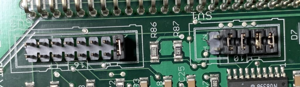
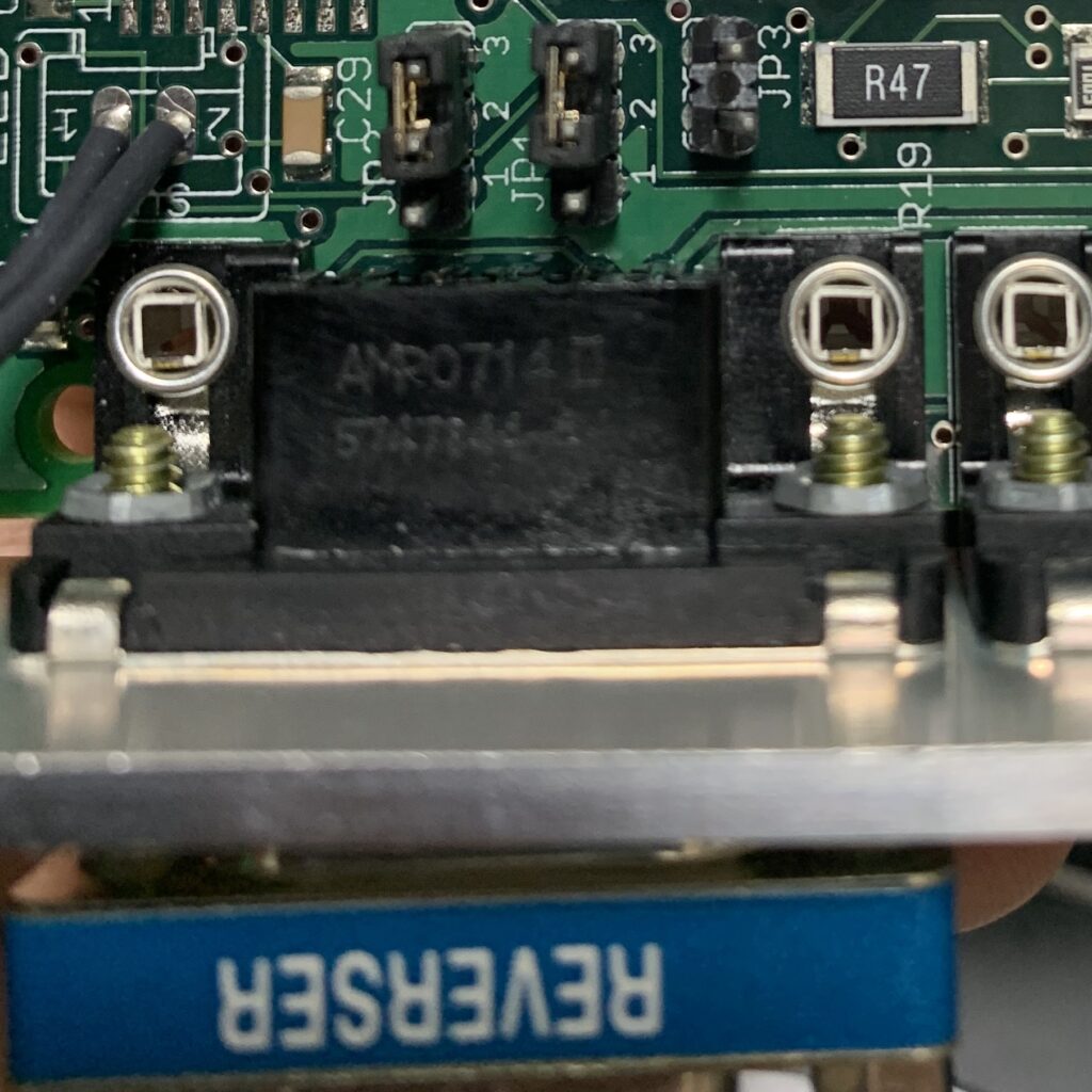
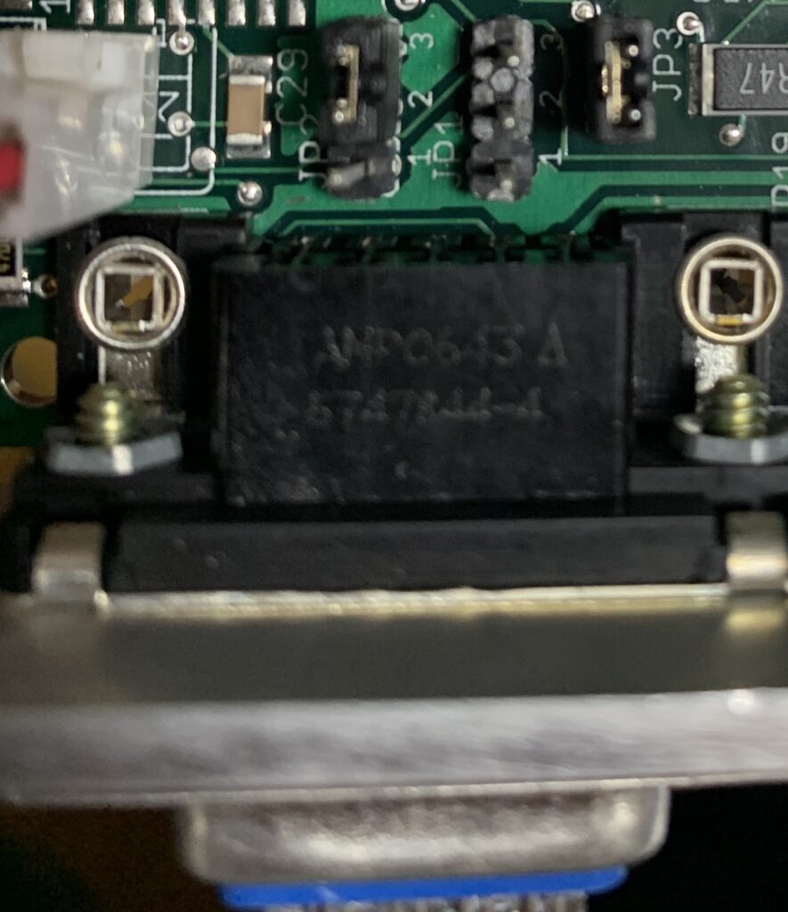
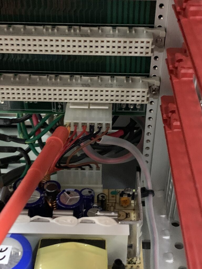
This is as far as I plan to take things in this post, but I may investigate the electrical side more later. In the mean time, below are a pile of pictures from the teardown:
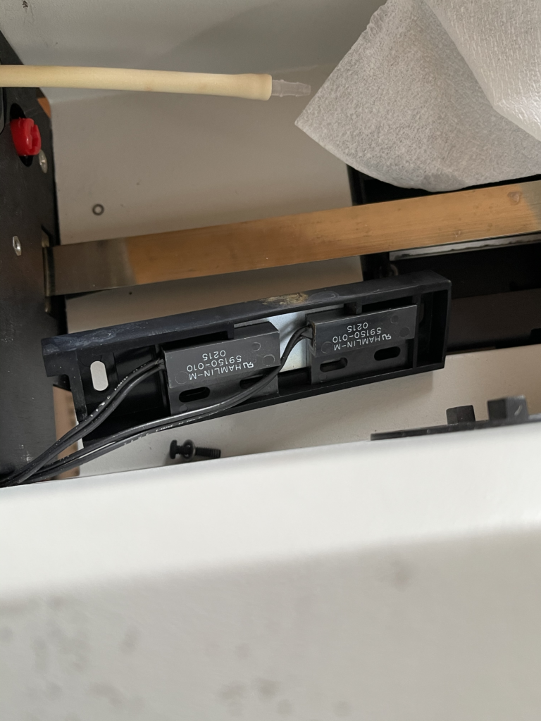
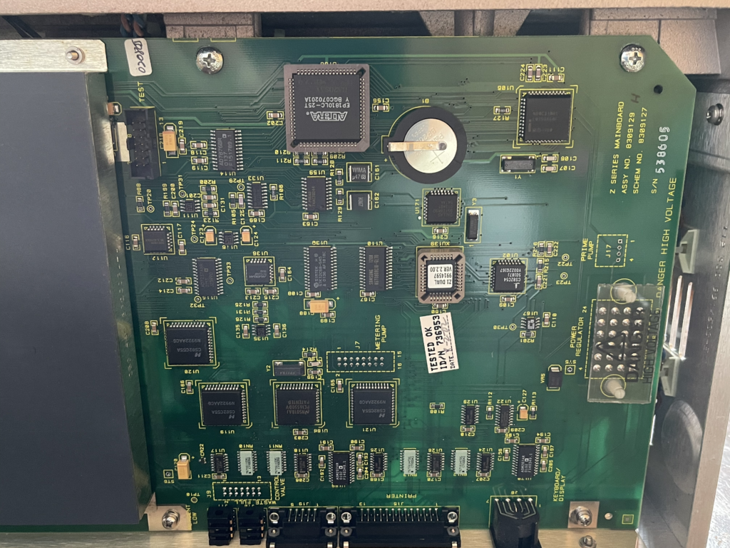
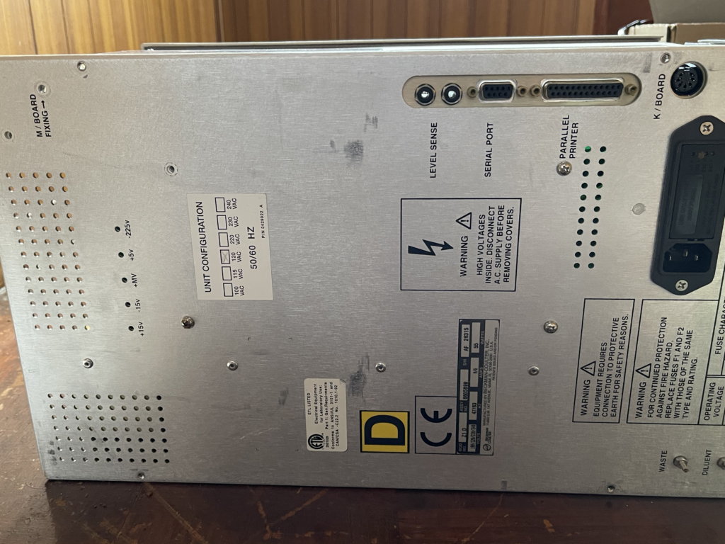
Genome Analyzer Quantum GEM 532nm Laser and filters

The Genome Analyzer contains two lasers. One of these is a Quantum GEM 532nm laser. Using an SMD 6000 driver. This laser is somewhat customized. Sam has some excellent info on these lasers.

In order for the laser output the following header needs to be attached to the “control” port (analog control input). This will not enable the output, but it will allow you to send RS232 commands via the serial port connection. The connection between 1 and 4 sets the maximum power output, a short will let you enter RS232 commands to drive the output to the maximum (550mW). A lower value resistor can be used to limit the power.

The laser can be controlled using the “RemoteApp Laser Control” software from Laser Quantum, which is a free download (or here). The driver doesn’t work well with the cheap CH340G based RS232 adapters that are generally available on eBay. So I recommend getting hold of a more standard compliant RS232 port.

Below shows the output of the laser when jammed against my self calibrated B&W spectrometer.

The genome analyzer contains an 8 position filter wheel. Only the first two positions are populated. The last two are blanked out. The “next” button on the LX4000 will only allow you to cycle between the first two positions (0 and 1). But the micromanger ASI filter wheel device will let you select any position (see previous blog post).

In my instrument the filter in position 0 is marked 1005190C 61009 ILLM-0027 Rev A. Jammed this against a Xenon light source and measuring the output with the spectrometer gives this rough spectrum:

Which suggests that this is a band pass filter from ~575nm to ~640nm (there’s likely a lot of stray light and reflections in my measurement).

The filter at position 1 is marked 1005271A A09369-309349 ILLM-0037 on my instrument. And gives the following spectrum in the same setup:

Which suggests this is a bandpass between ~540nm and 570nm.

Coulter counter/nanopore demonstrator

I wanted to knock together a quick visible demonstration of the nanopore/coulter counter sensing technique. This post documents a demonstrator using bits I had knocking around the house…

What is Ionic/Nanopore sensing?

(Ionic) Nanopores and coulter counters are devices that let you electrically detect the passage of small particles though a hole. The “hole” (pore, aperture) sits between two chambers which are filled with a conductive fluid. A voltage is then passed between the chambers and a current flows through the pore. Anything that passes through the pore blocks this current flow. So by measuring the current, you can detect the passage of particles through the pore. When a particle is in the pore, the current can’t flow as well as usual. So you get a short, drop in current as the particle blocks the pore.

Big particles block the aperture more than small ones. And you can therefore also get size information. This principle is used in the coulter counter to measure particle size distributions (for example to get white blood cell counts, or understand the distribution of particle in paints, or printer toner).

Building a macropore!

The basic sensing method described above works at a range of scales. All the way from millimeters down to nanometers. To get a feel for the basic principle lets build a macropore!

Roughly 2 to 3mm “pore”

I used a bottle cap, which I made a ~2mm hole in (I used an old soldering iron, but a drill would be better). The toothpicks in the side (completely blocking small holes), are to hold the “pore” in place later.

Next we need something to put though the pore. Most plastics are lighter than water and will just float and wont want to go through the pore. PMMA (acrylic) isn’t. But where I am it’s difficult to find PMMA pellets/granules.

So, with a pair of old wire cutters I cut up some acrylic sheet:

Then we can build our fludic system. We’re essentially going to build what was shown in the schematic at the top of the page. But there’s something missing, a way to drive particles through the pore. In this setup, we’ll use gravity.

The bottle cap will sit on top of beaker (or jar). It needs to be held in place, so the bottom of the cap with the hole in is completely submerged. But most of the bottle cap needs to be above the water line. If we add solution to the bottle cap it will then flow down into the bottom beaker.

For my setup I added a pump (cheap peristaltic pump from ebay) to recirculate the solution. Here’s the setup in schematic form. This is essentially the same figure as shown at the top of the page:

Below is the actual setup in all it’s glory! In my setup I used 1M KCl, about 7.5g of KCl in 100mL of DI water. I used AgCl electrodes (silver wire that’s been sitting in bleach for ~30mins).

I also needed to add a small barrier to help direct particles to the hole. Without this particles tend to get trapped in the fluid flow and spin in circles around the pore without going down it. I used a small piece of microscope cover glass:

You can then put a bias voltage across the electrodes and monitor the current. I used a oscilloscope to view the current trace. The scope has a built in function generator which I used to generate a 1v DC bias voltage.

Current was monitored using a self built transimpedance amplifier with a 1K feedback resistor. This was based around an LMP7721. But probably any FET opamp in a transimpedance configuration will work.

In the video above you can see the system working. As I pipette in some solution, you should see a small black particle fall down into the beaker. At roughly the same time, you should see a small upward “blip” on the oscilloscope, as the particle translocates the pore.

The PMMA particles tend to float on the surface tension. So I’m pipetting solution on top of the particle to make it sink.

Hopefully this provides a basic visual demonstration of the “pore” or coulter counter sensing approach. If you’re interested in ionic sensing, you should signup for Demonpore. Demonpore is making a molecular gaming platform which lets users experiment with pore based sensing. And my desire to experiment with macropores here comes out of discussions we’ve had around explaining nanopore sensing in visual and compelling ways.

LX-4000 stage controller notes

The LX-4000 is the stage controller used in the Illumina Genome Analyzer 2. It’s a custom stage controller made by ASI somewhat similar to their ASITiger controllers. The controller is essentially a chassis with a backplane providing power and common bus to expansion cards. This post contains my notes on using this controller.

The LX-4000 contains 3 cards. The FW-1000 (filter wheel), a “Z/F” card (Objective, Z-axis), and a “X/Y” card. The “Z/F” and “X/Y” cards are essentially the same design. These PCBs are labelled “Two Axis Board” on my device one is “REV. C” (the X/Y) and the other is REV. D.

Communication

All 3 cards have ports that look like RS232 ports, only the port on the “Z/F” card can be used to communicate with the device. Commands for the other cards are routed over the internal backplane.

The FW-1000 card has a port labelled “RS-232” on my instrument this is not physically connected to anything. The filter wheel can be controlled manually by pressing the “NEXT” button or via the “Z/F” serial interface.

A CH340 based USB serial converter works well with the LX4000. Many CH340 RS232 converters work quite poorly, seemly mostly on the transmit side. A number of issues I had with getting the LX4000 to work with micro manager were caused by the device only registering some of the commands the CH340 was sending. I therefore recommend getting a better USB serial adapter. The Edgeport 8port serial card supplied with the Genome analyzer works well. Probably a (real) FTDI device would work well too.

The USB-serial adapter should be attached to the usually included “Reverser” (I believe a null modem converter). Baud rate is 115200 (8N1) on the “Z/F” card.

When powered up the serial will output “F” or “FX”. It may also report “MOTOR 1 NOT RESPONDING” or similar. This indicates that only one filter wheel is installed, and is not an error.

The general command set seems to follow the MS-2000 protocol.

While the instrument is initializing it’s possible to enter serial commands such as “1H I Z”, which will return information regarding the Z axis. However after a few seconds the device will start replying with “BELL”s (or possibly just in hex). I had issues getting the device to respond here.

However, the ASI TLX4000s.exe application will happily communicate with the controller and control everything except the X/Y stage without further modification (see notes on the X/Y stage below).

The LX4000 command set seems to be similar to the MS2000. However commands need to be prefix to address the required stage as follows:

1H: z stage
2H: x-y stage
3F: filter wheel

Micro manager is supposed to support the LX4000, but depending on the version you have you may have issues. I found that initial setup with the ASI software is most reliable. This software is a single exe called “TLX4000s.exe”, available from this excellent blog post on the GA2 ASI stages (or local copy). The software is somewhat troublesome to get working on modern systems and appears to have been written in Visual (Basic?) 6. The various runtime library either don’t work, or don’t include all the necessary components for Windows 10. My route to getting this working was to create a Windows 7 VM, then install Visual Studio 6. This doesn’t take long and insures that all the necessary libraries are installed.

In the genome analyzer the socket labeled “LIN ENC” on the X/Y card is as I understand it connected to the door sensor. The only pins connected on the genome analyzer are pins 5 and 8. This seems to provide a hardware lockout on the X/Y stage when the door is open. The following image shows a 1K resistor between these two pins, and when connected to the “LIN ENC” socket will allow the X/Y stage to operate. Take care when creating/installing this as shorting the wrong pins can damage the X/Y card (see “Cards” below).

Without this is place, the X/Y stage will not move on my unit, the Z stage and filter wheel will however happily work.

I was able to get the LX4000 to work with micromanager 1.4 and 2.0 (1.4.23.20160628 and MMSetup_64bit_2.0.0-gamma1_20210309). But things seem fairly unstable (much more stable with a good USB serial adapter, but auto-detection is still problematic). You need to add the following devices: XYStage/ASIStage ZStage/ASIStage and ASIFWController/ASIFW1000. Sometimes stages were detected correctly, sometimes not… (my config is here). I generally had to enter the COM parameters directly, scanning was not reliable.

Cards

It’s wise to be careful when shorting pins on the jumper connector shown above. Shorting the wrong pins dumps (likely RS232 level signals?) possibly on to the 5v power rail, or elsewhere. It’s possible to kill the card by doing this.

If this happens, it will likely blow a 5v trace near the expansion card connector. This traces are very thin and act like fuses… I’ve done this… repairing the trace seems to fix the card…

Repaired 5v power trace…

All the expansion cards seem to use Silicon Labs MCUs. C8051F122s on the two axis cards. C8051F015 on the FW1000.

The two axis cards uses TDA7269As to drive the stages.

Card communicate across the internal bus. The Z/F is the controller. If the Z/F card is not present the FW-1000 and X/Y cards will not come online (the LEDs and displays will not illuminate).

Jumpers SV3 and SV1 on the rear of the Z/F card control how control signals are routed across the backplane. If they are not present, the other cards will not come online. Here’s the default jumper configuration:

Here’s the default jumper configuration for the XY card:

There’s also a set of jumpers near the serial port. If these are set incorrectly you will experience varying degrees of weirdness (seems to still work in some configs, but outputs a lot of extra stuff). Here’s my config for the Z/F card:

And for the X/Y card:

Filter Wheel Config

The filter wheel can be configured with the TLX4000s.exe application (see Communication above). This can be used to change the filter wheel offset if it comes out of alignment. To do this, open the software, select “Filter Wheel” (after establishing communication). Then change the slider at the bottom of the “Filter Wheel Command” window. When you have adjusted the offset click on “RS” (Ram Save) which save settings so they are stored across reboot. The offset can likely also be adjusted using the “OF n” command where n is an offset, though I’ve not tried it.

The filter wheel has 8 positions (two of which are blanked out). The “Next” button on the LX4000 will only select between the two populated filtered. But serial commands can be used to move between any filter position. Micromanager supports this (use the ASIWheel device, and create groups to control filter wheel presets).

Power

The backplane provides +/- 15v, 5v and 24v to all cards. A 6 pin connector provides the +/- 15v and 5v supplies to the backplane. A second 3 pin connector supplies 24v.

In the image below the probe is on the 15v pin and from left to right voltages were probed as:

15v 5v 5v 0v 0v -15v

The connector to the right of the 6pin power connector is the 24v connector, on the opposite side of the board. This is supplied by a separate power supply that sits at the rear of the device (Condor GPFC110-24). In the orientation shown in the image below this reads as 24v 0v 0v.

Power is distributed to the expansion cards via the 8 thick traces shown in the image below on the right side of the expansion card. The last 8 traces probed as:

15V 5v 0.5v 0v 24v 0.2v -15v 0v

With the voltages <1v probably being measurement artifacts due to poor probing/grounding.

Pasted Graphic.tiff

Of the 3 pins holes across the expansion connector, the central pin is not fitted. The pins on the edge (“top” and “bottom”) of the connector as connected. This is true for both the power and data lines.