I picked up an IMX178 based camera. These cameras are cheaper than the IMX174 based ones, have smaller pixels (bad) but better noise specs. Images generally looked a little better (the image below is atto1178_5) with used 1s exposures and 4x binning:
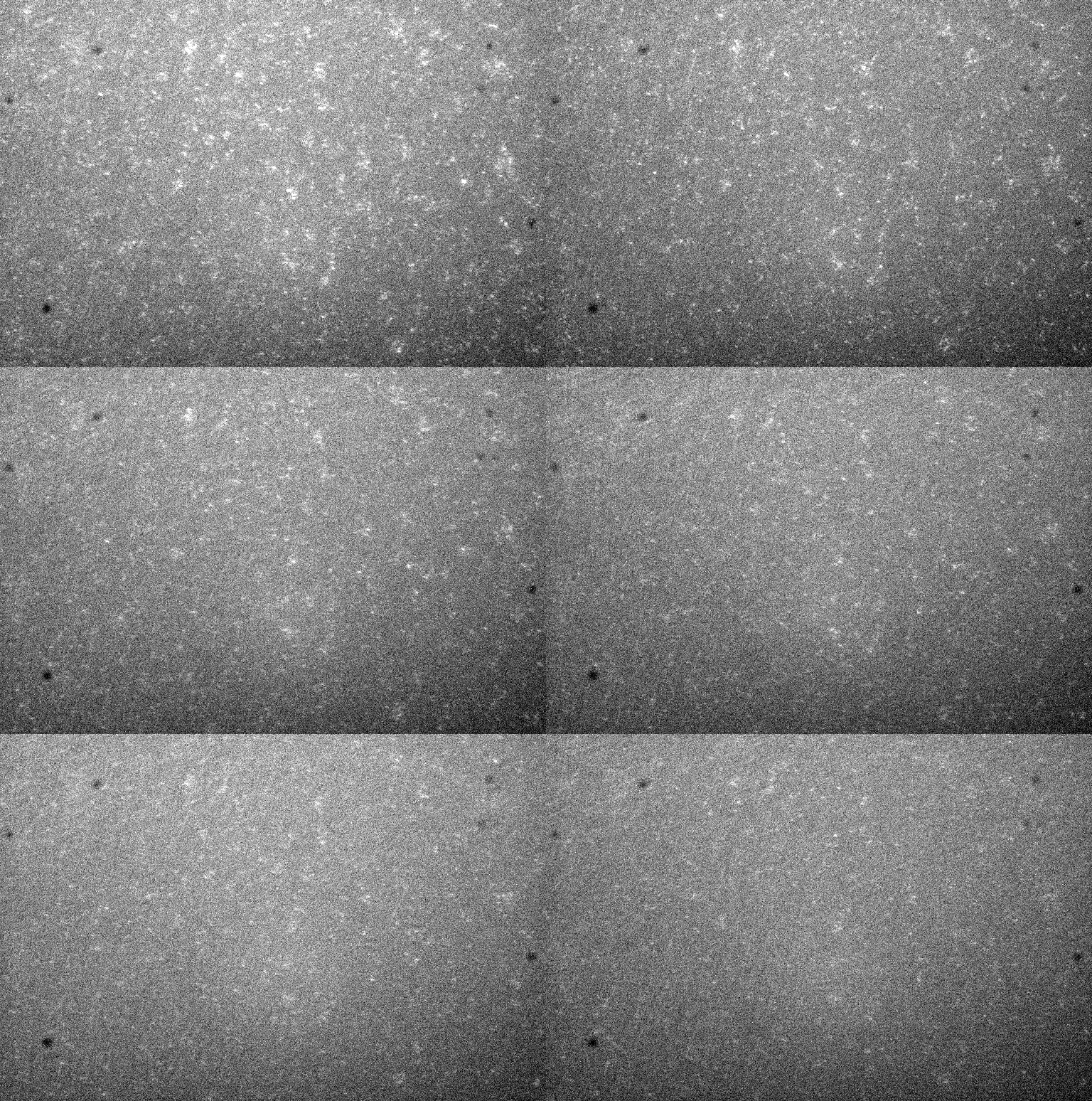
But I found turning the mode scrambler off produced much much cleaner images, with better defined points. However, this introduces the “wavey” illumination that you can see in the images below (500ms exposures here, atto1178_13):
Turns out the mode scrambler (which works by vibrating after all) was causing a lot of vibrational issues. While the mode scrambler is attached to a dampening mount, I found that stuffing a pile of kimwipes under the unit, cleaned up more of the vibrational noise:
The results are reasonably clean (Atto1178_21, 2s exposures, binning=4):
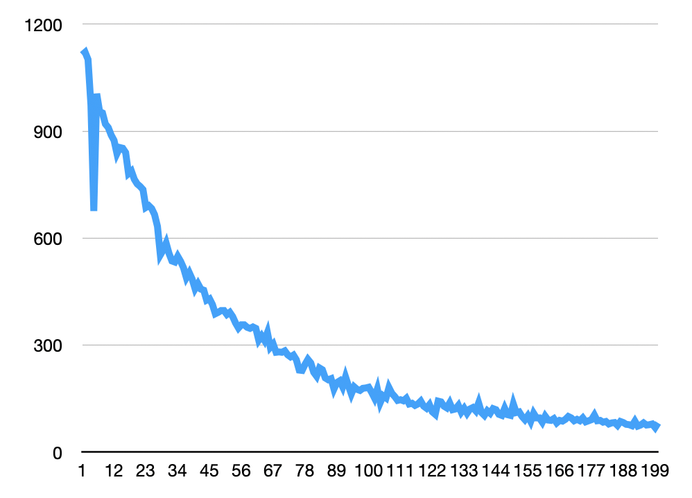
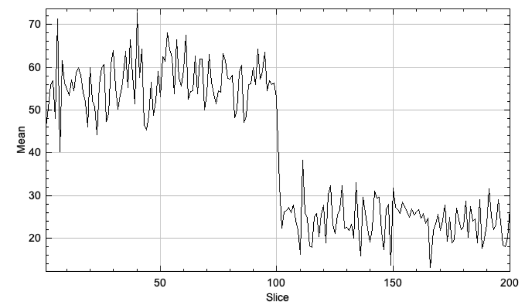
With some basic thresholding, I was able to quickly extract particles from this dataset in Fiji. In general for the images above I enhanced contrast (using the stack histogram) and background subtracted (default values, 50px window). Below I used analyze particles to generate particle counts on a manually thresholded stack (same thresholds were used for all images). These looks more or less as expected for a photobleaching experiment, with the dip at the beginning caused by the image becoming saturated/some spots colliding:
You can also pick out fairly clean traces across frame for spots that bleach (Plot Z-axis profile over a spot):
Not much is publicly available regarding Ultima genomics. The company appears to have received >3M USD in SBIR awards in 2019 and 2020 (which is by usual standards, rather a lot). Its CEO is Gilad Almogy who was previously CEO and founder of Cogenra (a solar company). Aside from this I can’t find much information about fund raising. The company appears to have been founded in late 2016. From the SBIR application, and patents it seems clear that they are focused on DNA sequencing.
Technology
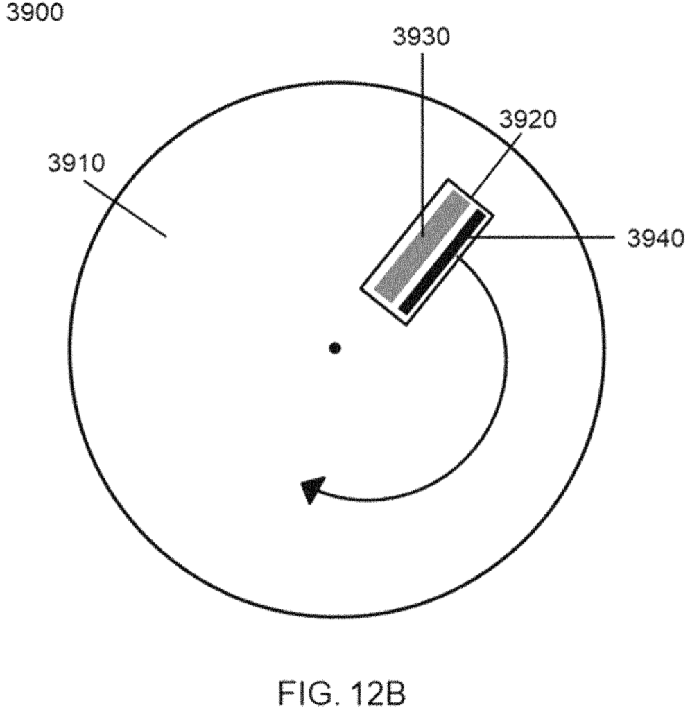
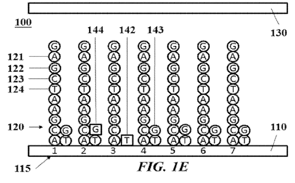
I’ve taken a very brief look at a couple of Ultima’s patents. The first patent describes an imaging system for use in with a DNA sequencing platform. The substrate is on a rotating platform:
Which is somewhat reminiscent of Ling Vitae approach. Where a fluidic system was incorporated as part of a CD-like platform. I kind of like this idea, because you can potentially image a large area, with one stable axis. After an imaging pass, you end up where you started, ready to image again. In a cyclic sequencing approach, this seems attractive.
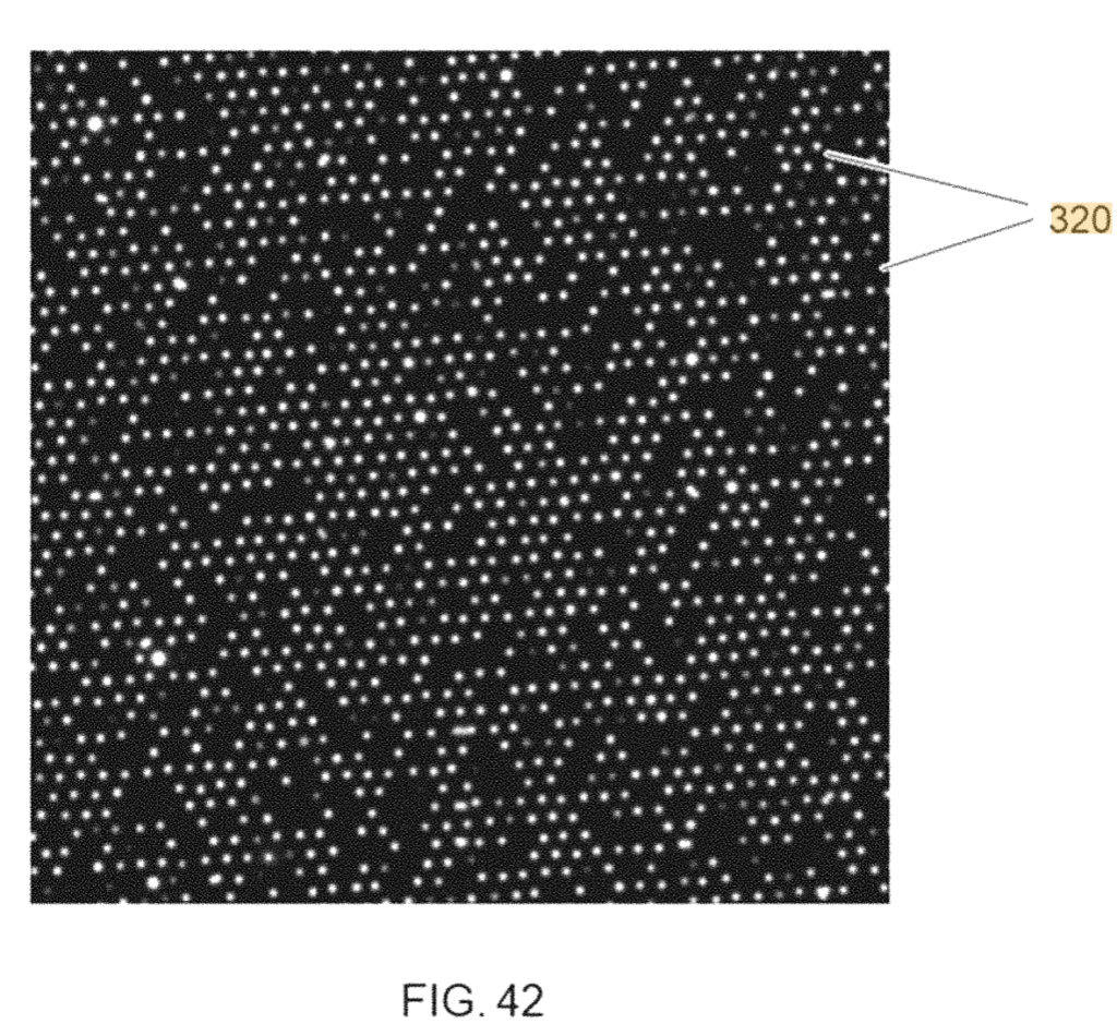
The patent also shows what looks like real image data from an ordered array:
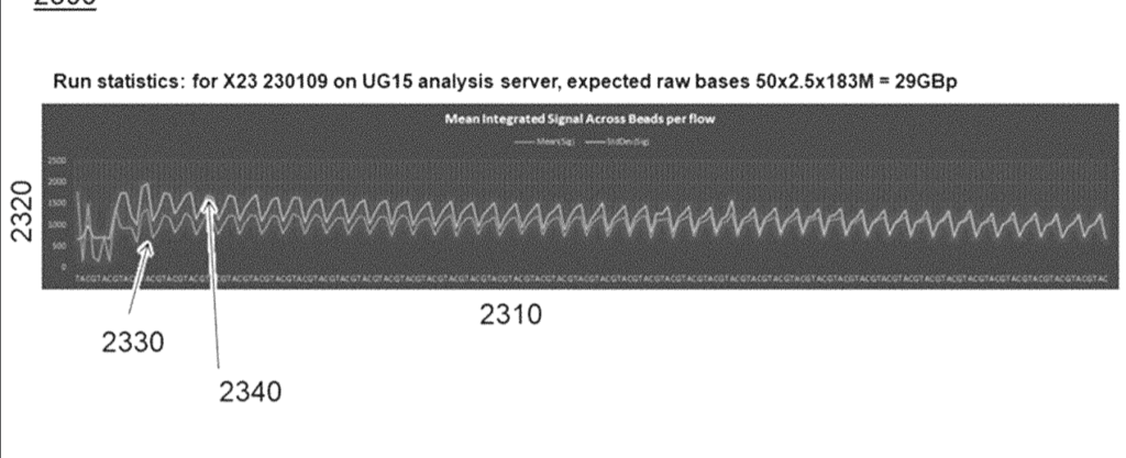
And even some read statistics. I’d need to read this in more depth, but I suspect this is just extrapolated from spot counts:
This is also not a traditional single-channel/unterminated SBS platform (Ion Torrent, 454), which would incorporate a single base type in each flow.
The Ultima Genomics approach presented here, works on a population of templates (so a surface amplification approach like cluster generation, or a bead based approach would need to be used).
In the dominant embodiment, it appears that Ultima Genomics would incorporate mixtures of terminated and unterminated bases. Most positions would extend normally using a wildtype nucleotide. However a smaller fraction of nucleotides would be terminated, preventing templates from extending any further. These terminated nucleotides would be labelled (likely a fluorescent label). Allowing the sequence of a cluster to be determined from the terminating sub-population.
One obvious issue with this approach, is that with each cycle, you get an accumulation of incorporated dye. You could cleave the fluorescent labels, which seems like the obvious thing to do. But the patent suggests a different approach, essentially just monitoring the increase in fluorescent intensity. An increase in a cycle means that a base was incorporated, no increase – no incorporation.
That’s fine as it goes, but eventually the build up of dye is going to make imaging problematic. You’ll either overflow the cameras range, or get increased crosstalk from scattering etc.
To avoid that one suggestion in the patent is to periodically switch dyes. That is just move to a different dye with a different emission after a few cycles. You can then switch filters, effectively cutting out fluorescence from the accumulated dye.
Overall some aspects of this approach don’t seem particularly new. Using terminators was of course the foundation of the original Sanger sequencing approach. And mixtures of nucleotide types have previously been used for sequencing in academic work. Some of this prior work may explain why the majority of claims on this patent have been cancelled.
The chemistry itself seems more complex than those currently available… so what is the advantage? I suspect the motivation is that wildtype bases likely incorporate more efficiently. This might give some improvement over Illumina-style SBS. The fact that platforms using wildtype nucleotides (Ion Torrent, 454, Sanger) have somewhat longer read lengths (on the order of 1000 nucleotides, versus 150) supports this.
But in this Ultima approach, the loss of templates through termination will eventually limit read length. It’s also worth noting that while the other platforms mentioned above have longer reads (and in some cases lower error rates) they have not proved commercially very successful. So I’d be concerned that the added complexity of the Ultima approach doesn’t provide enough benefit over existing platforms.
That said, this is only a quick review of a couple of patents. I will be watching with interest to see how things develop.
I’ve been playing with an old Genome Analyzer 2. This post documents my first attempts to see single dyes, and results which I suspect maybe single dye photobleaching. Hopefully I’ll get round to documenting the rest of the system in another post.
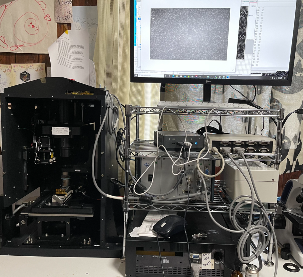
This setup uses the 532nm Quantum GEM laser with a Nikon ELWD 40x DIC (not used for DIC) objective. A 60x ELWD is likely preferable, but this used objective was only ~400USD, cheaper than any 60x I’ve found. The stock camera has been replaced with a cheap monochrome IMX174 (ZWO ASI174MM). This commodity industrial sensor has been used in other single molecule studies. The genome analyzer uses an ASI stage for XY and Z axes, which works with micro manager.. The Quantum GEM laser was controlled using their software. The ZWO camera has a plug which works with micro manager 1.4. Images were taken using the stock Illumina filter (at position 1), this appears to be a long pass filter from ~540nm.
I’m using Atto 542 NHS-ester (AD 542-31). I serially diluted Atto 542 in Ethanol ~16 times diluting by a factor of >40 each time, i.e. less than 1^10-16 of the original concentration. Essentially I pipetted <10uL of solution into 400uL.
I then pipetted ~10uL of the final solution onto 18x24mm cover glass (Matsunami Glass Ind. Ltd.). This took some experimentation. I don’t believe the dye dries evenly on the cover glass. If any kind of residue was visible by eye this indicated that the concentration was too high, and I diluted further.
The prism was cleaned with Ethanol/Kimwipes (likely not ideal). I placed a small drop of Cargille #19569 fused silica matching liquid on the prism. And placed the slide on top of this (after evaporation of the ethanol). The TIRF laser and objective had been previously aligned (which I will describe in another post).
I tried a variety of exposure times, camera settings, and laser powers. I could eventually see something reasonable using the full laser power (550mW), camera binning of 2, and 2000ms exposures, 8bit. Below is an initial capture, where you can see individual “spots” blinking off.
I process this with ImageJ/Fiji. Running a Kalman filter over the image, applying background subtraction, normalization, removing small particles etc. until I could pick out somewhat reasonable spots on the thresholded image. The data is pretty noisy and there are a number of artifacts…
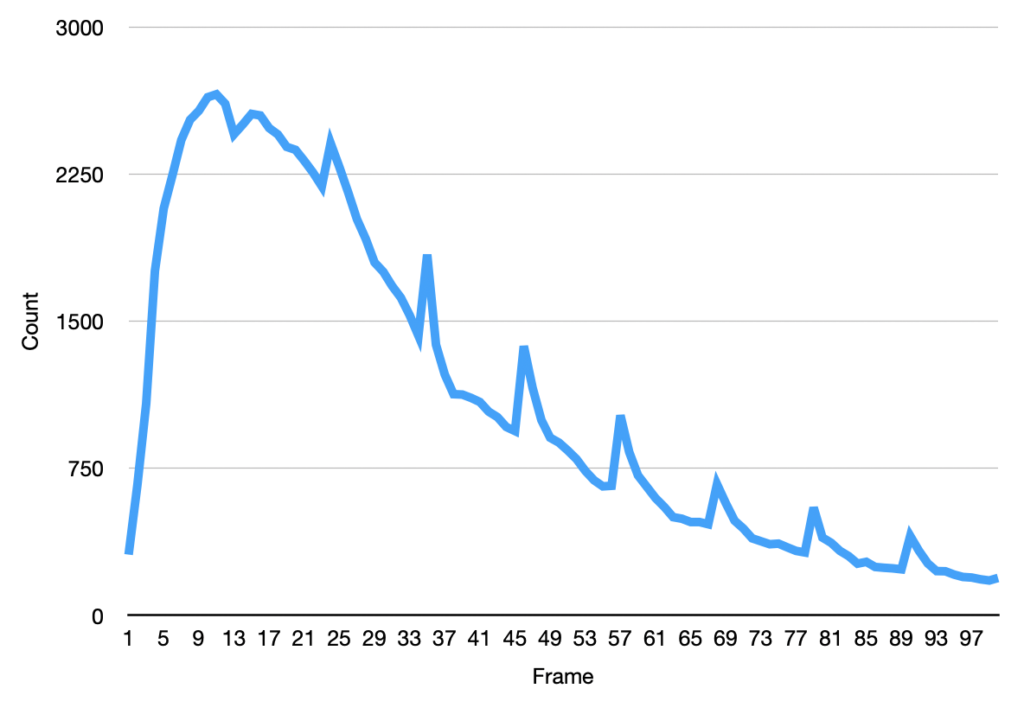
I then ran this though the “Analyze Particles”, to get particle counts…
The initial frames don’t process correctly (the image is too saturated with spots, and the particle identification doesn’t work correctly). This causes the initial “slump” but from around frame 13 we see a roughly exponential decay. This seems consistent with single dyes. Why we see periodic peaks is less clear. I suspect this is spike noise (as we clearly still pick of false particles in the thresholded images). At higher framerates you can sometimes see the laser intensity pulsing, and I suspect this is an artifact of that.
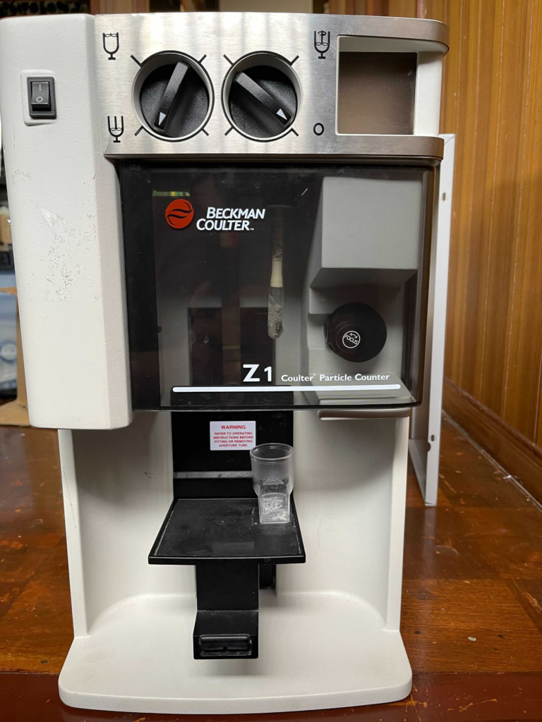
I picked up a Beckman Coulter Z1 particle counter on eBay. I suspect it was non-functional. The control pad was missing and the rear case only had one screw. But this was fine for me as I was mostly interested in pulling it apart.
I’ll cover the aperture and fluidics first here. A dump of the pictures of the rest of the unit can be found at the end of this post.
Coulter counters are used to measure particle sizes. For example, to gain red and white blood cell counts. They do this by suspending particles in a conductive (salt) solution. This fluid is then driven through a aperture. A bias voltage is passed over the aperture and the current flowing through the aperture is measured. The fluid is driven through the aperture under pressure. As particles pass through the aperture they block the current flow, and can therefore be detected/counted.
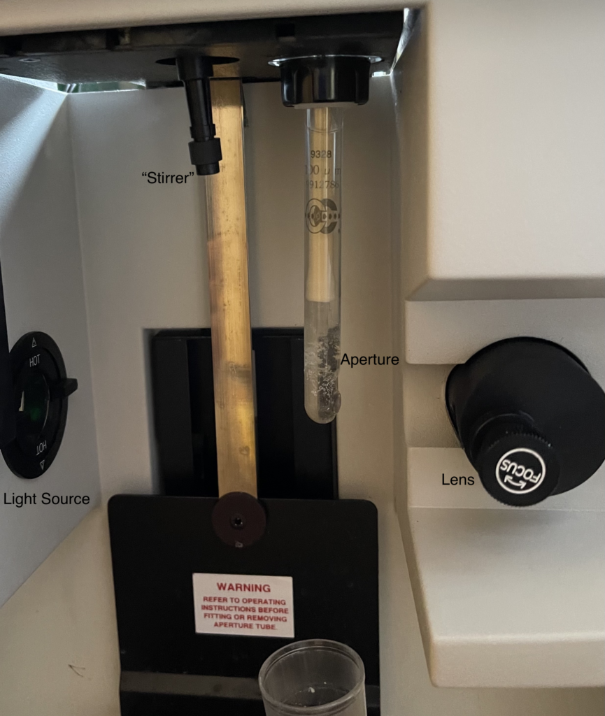
The aperture “rod” screws into the unit. There’s a light source (Mercury lamp I think) which can be used to illuminate the aperture. This is focused through the lens on the right and projected on to a screen at the top of the unit. The system is purely optical, there’s no detection electronics. It’s unclear to me how clear the alignment of the aperture is… or what the exact purpose of optically monitoring the aperture is.
There’s a stirrer attachment to the left of the aperture rod. From the rest of the system I suspect this also makes electrical contact with the fluid.
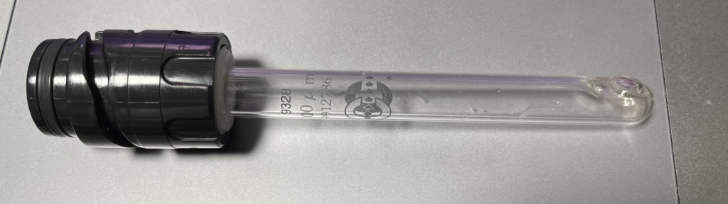
The aperture rod itself is a glass tube:
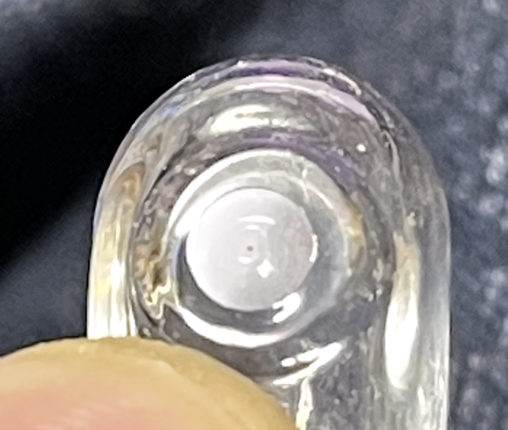
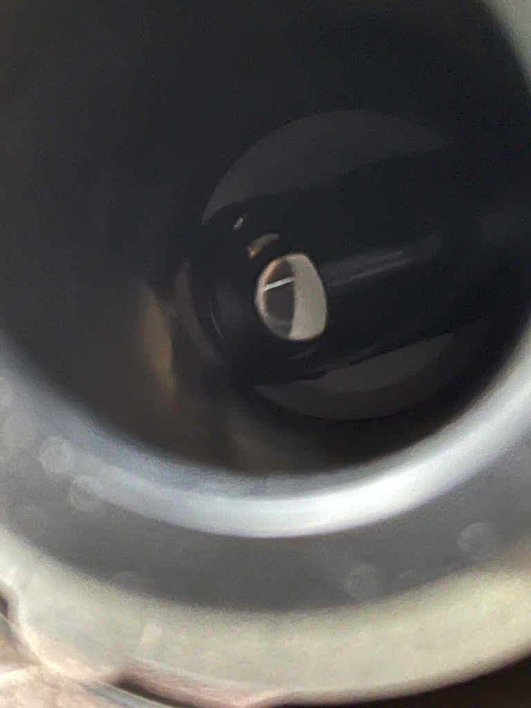
At the end of the tube is a flat disc with a small aperture in it. It’s not clear to me if this is a polished part of the glass or a disc embedded in it:
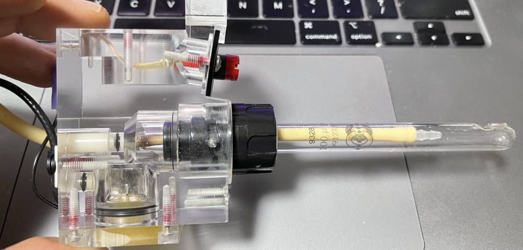
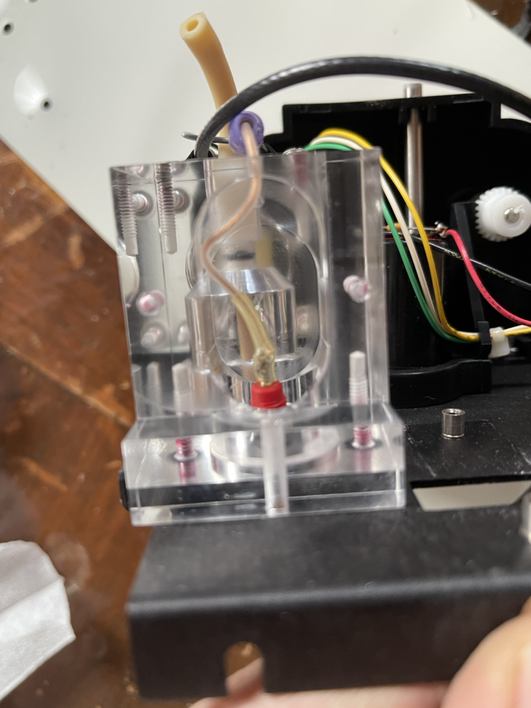
If you pull apart the instrument, you’ll find the aperture attaches to a small fluidic block:
The coax cable on the left makes contact with the foil sheet on the bottom (with is in the interior tube fluid path) of the unit and the red connector on the top of the unit. Somehow this top red connector must make contact with the sample. I assume via the stirrer…
There are two fluidic connectors at the top of the block. I imagine the instrument can pre-fill the tube via one of these.
Fluidics
The bulk of the instrument is composed of two fluidic components. A selector valve, and a metering pump.
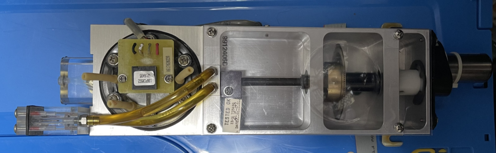
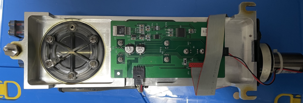
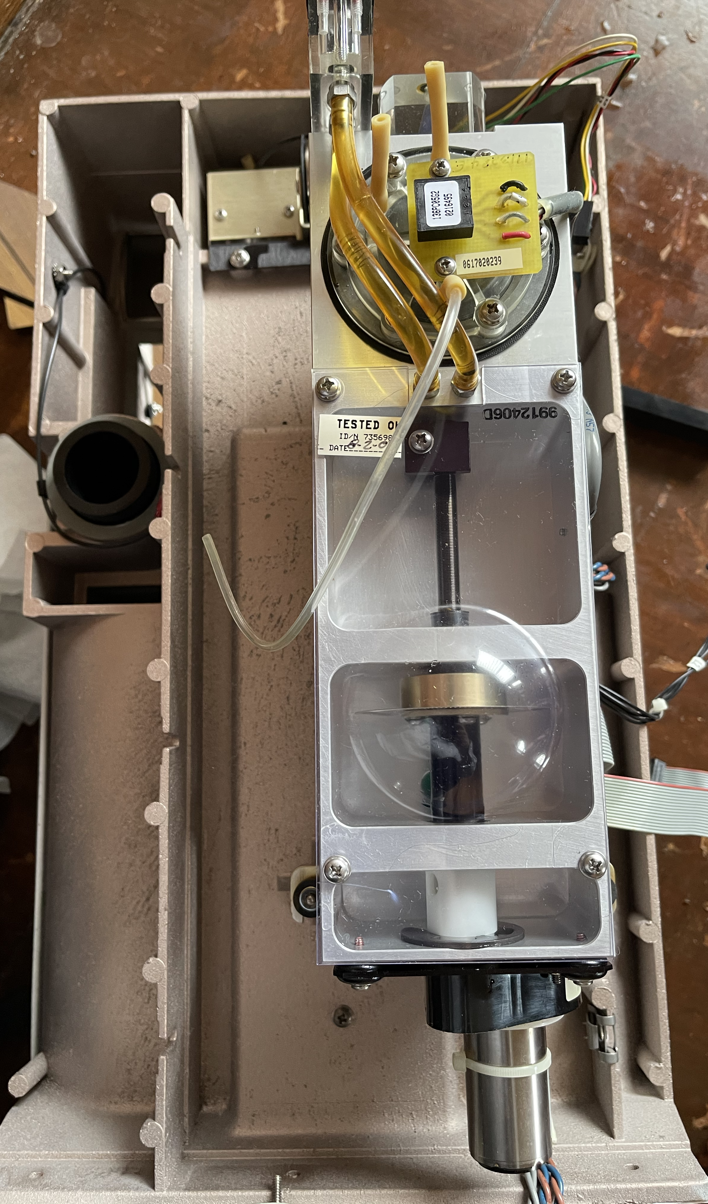
The metering pump, labeled “Metering Module”. Is a rather attractive piece of engineering:
Pump “front”
Pump “rear”
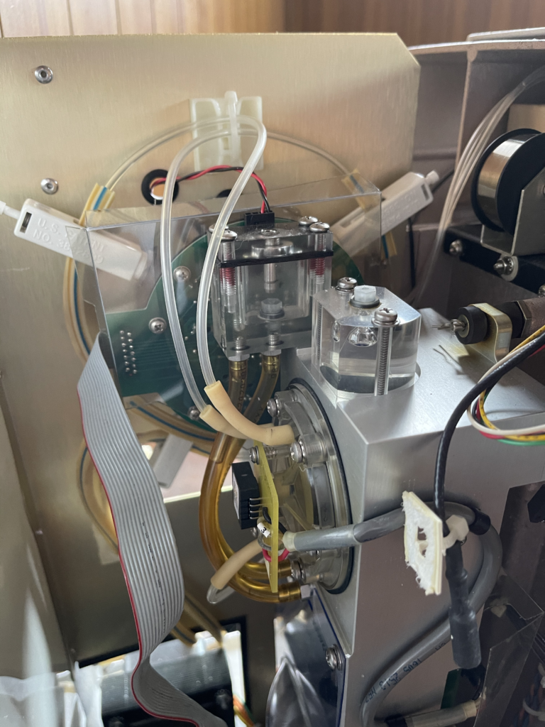
It appears to essentially be an oil filled diaphragm pump. On the “front” of the unit above you can see a Maxon DC motor to the right. This drives a rod with an encoder wheel on it. The rod feeds through into the oil chamber.
By pushing the rod into the chamber the oil push pressure on a membrane which can be used to move fluid around…
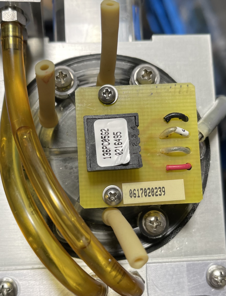
This membrane makes contact with the fluid on the other side of the pump (“front” above”):
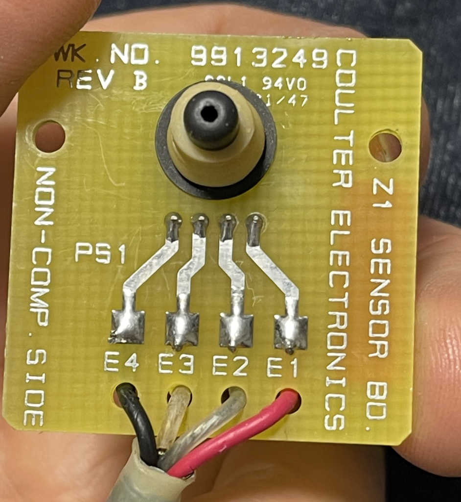
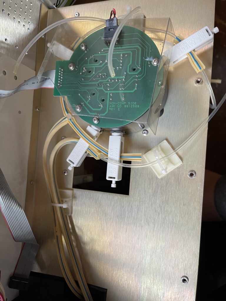
The three fluidic connectors/tubes above all make contact with the main chamber containing the diaphragm. The component on the PCB above also makes contact with the chamber, and I would guess is almost certainly a pressure sensor:
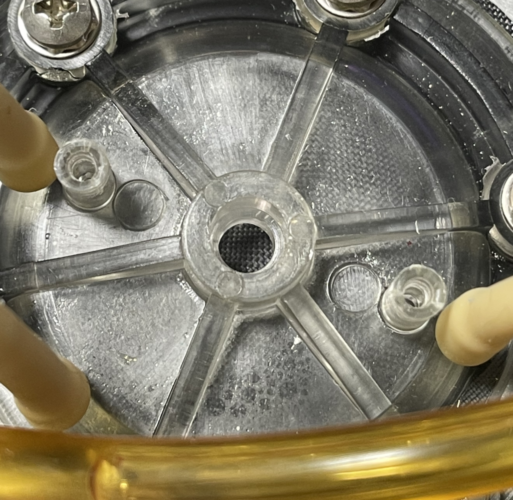
With the pressure sensor removed you can just see the membrane:
As it goes, this is all fine. But in order to move fluid around, the diaphragm pump needs a valve to open and close the inputs/outputs. In a regular diaphragm pump these are usually mechanical valves:
But in order to allow the pump to switch between different inlets/outputs the Z1 uses a motor driven selector valve:
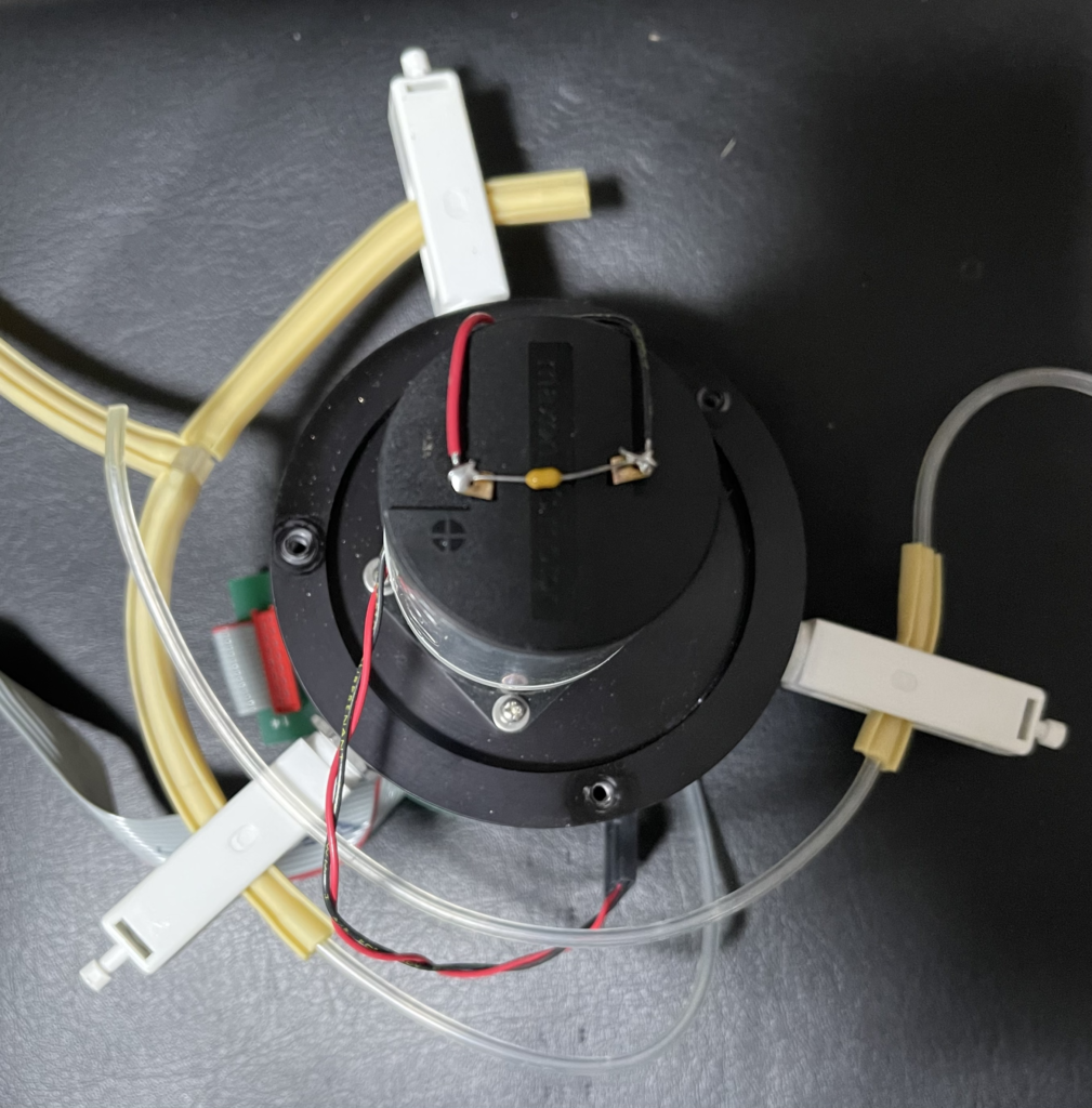
This is a very simple mechanical system. The white valves just clamp tubes shut under pressure:
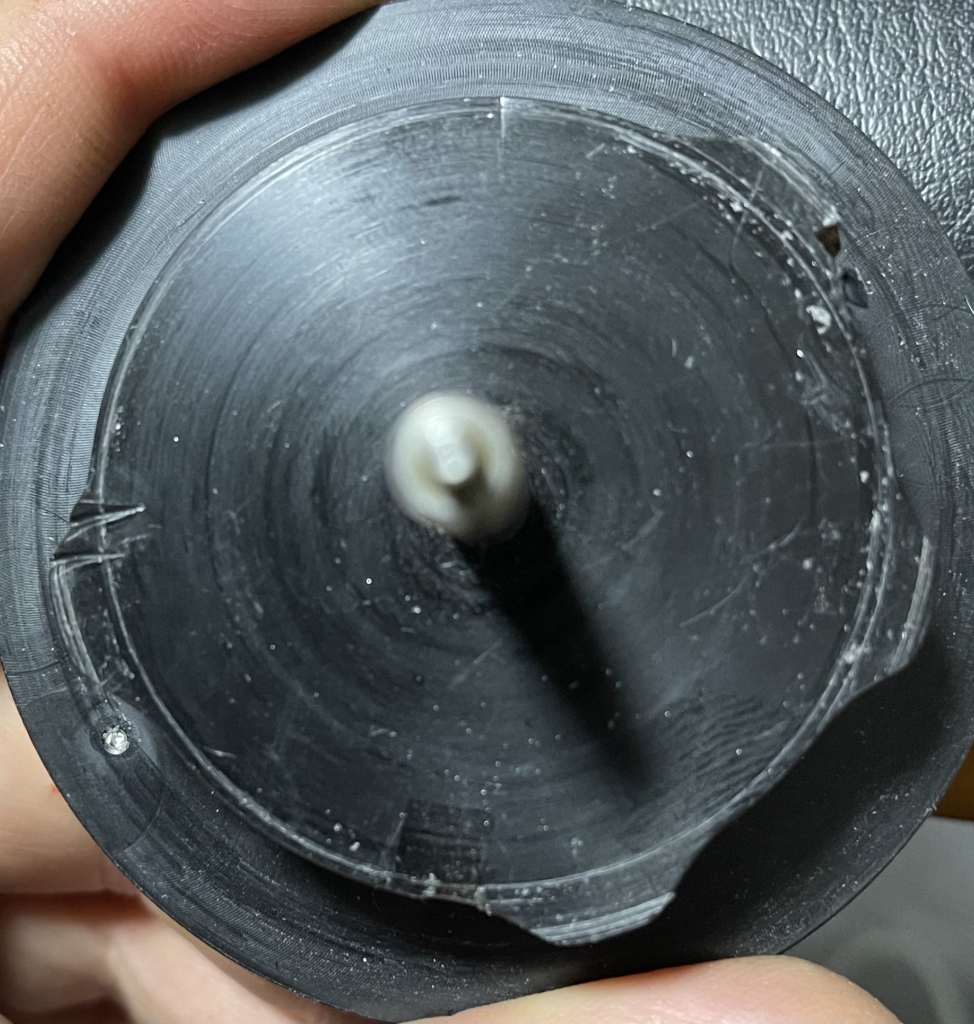
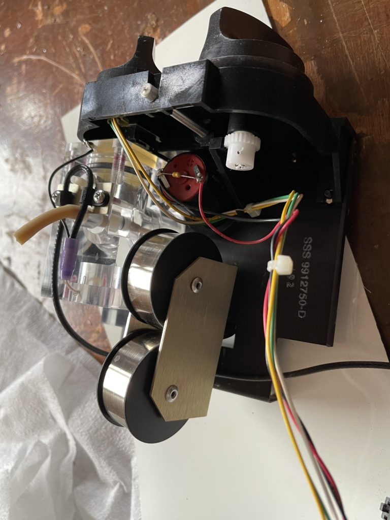
Inside the unit is a wheel which is rotate by the motor to put pressure on the values:
For the most part this wheel seems to clamp down on one valve at a time. So I would imagine this can be used to first fill the pump chamber with buffer. Then clamp off the buffer, and allow the pump to fill the aperture tube. Then pull fluid through the aperture tube into the pump chamber before finally ejecting it to waste.
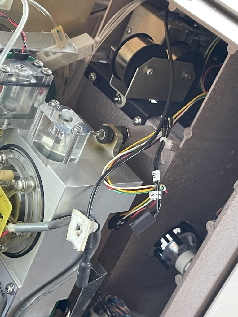
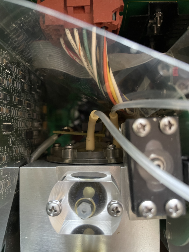
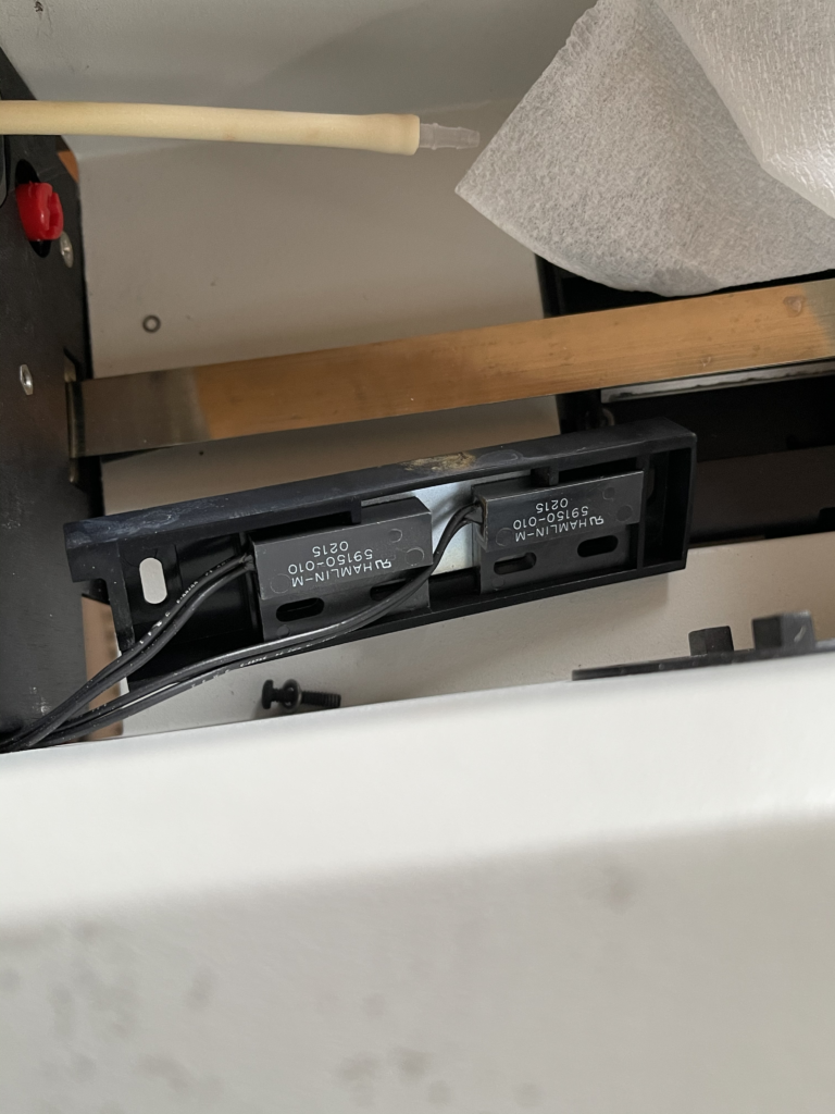
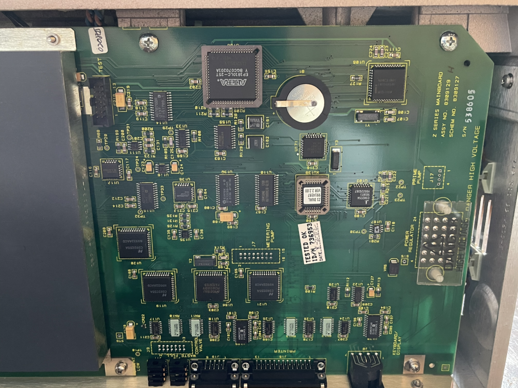
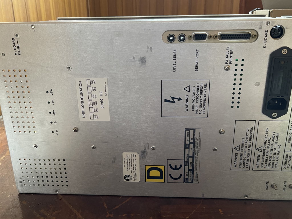
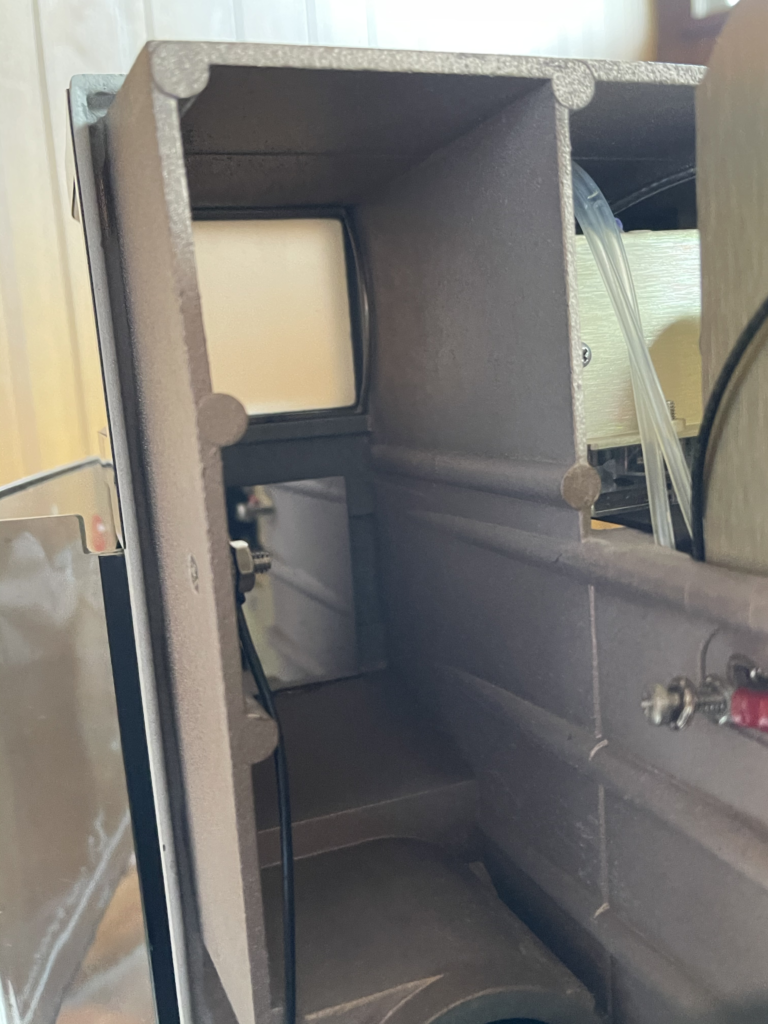
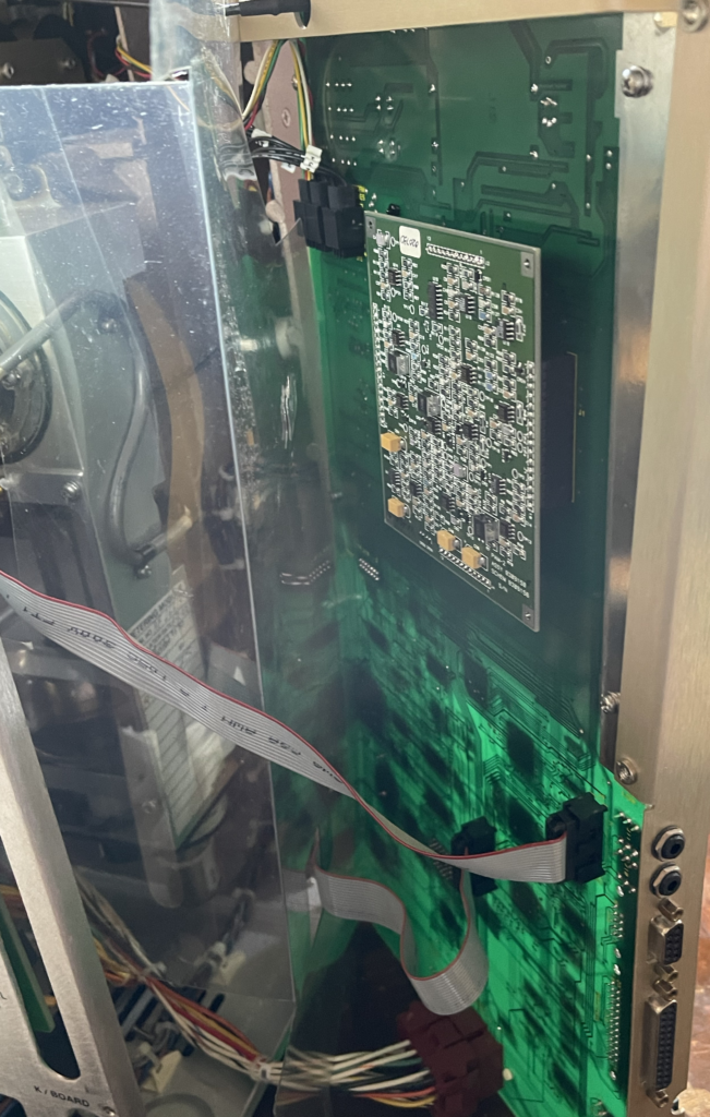
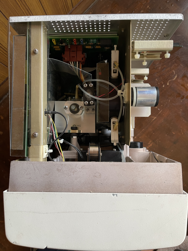
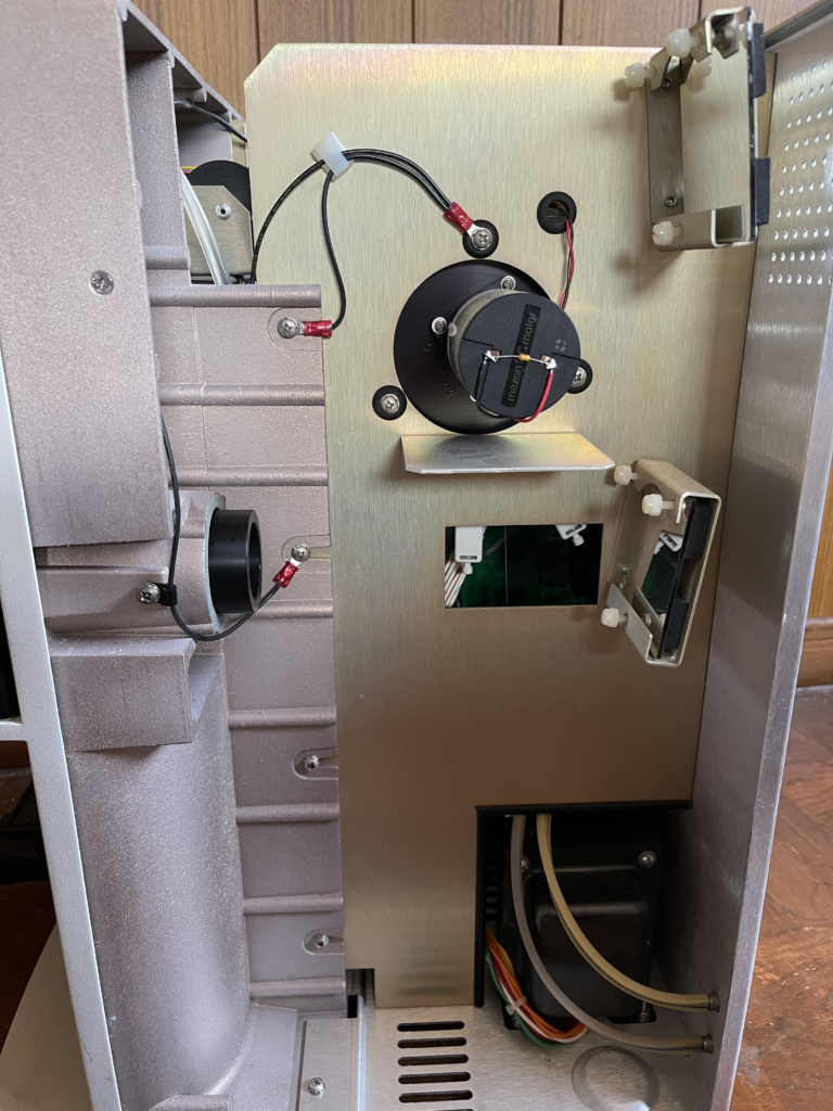
This is as far as I plan to take things in this post, but I may investigate the electrical side more later. In the mean time, below are a pile of pictures from the teardown:
My name is Nava Whiteford. I’ve worked for a few sequencing companies. I have equity in a few sequencing companies based on my previous employment (I try to be unbiased in my posts). You can contact me at: [email protected]





 RSS
RSS