The Solexa Pipeline
Some old notes on the Solexa pipeline, some of which may still be relevant. The latex conversion of this document is a work in progress, so bare with me.
A pdf version of this document is available here: pipeline
Firecrest
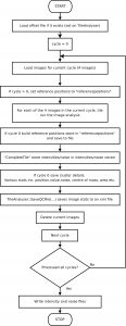
By default Firecrest operates on a per tile basis, the main Firecrest binary is run_image_analysis. It reads an xml list of absolute paths to tile images. These are created by Goat and stored in the Data/CX-CC_Firecrest1.9.2_DD-MM-YYYY_username/Firecrest/LXX/s_X_XXXX_XX_jnl.xml files. The main Firecrest loop is shown in figure 1. The main loop is largely straightforward. Firecrest loops over all cycles (typically 36) and then performs image analysis on each of the four images for this cycle. The image analysis identifies clusters, and the intensity and noise values associated with these. In the first cycle cluster reference positions are stored (later cycles are aligned against these positions).
firecrest-loop
\section{Firecrest runs in 2 passes}
When Firecrest is launched by the Makefiles in the runfolder it is called twice per tile. The first pass runs a full image analysis on every 50th tile. It’s “useful” output is an offsets file. This file specifies transformations (shift and scaling) that are applied to image data in the second pass.
The offsets file is created from the xml output of the first firecrest pass. These are stored in
(\texttt{Data/CX-CC\_Firerest1.9.2\_DD-MM-YYYY\_username/Firecrest/LXX/s\_X\_XXXX\_XX\_qcm.xml}). When the first Firecrest pass has finished \texttt{parse\_offset\_scaling.py} (a part of Goat), is called by the Makefile. This strips the scaling/offset data from the xml files are stores them in the \texttt{Offsets} directory on a per lane basis.
\texttt{update\_offsets.py} is then called. This file creates \texttt{default\_offsets.txt} which contains transformations which will be globally applied to identified clusters on the next Firecrest pass. It creates this offsets file as an average of the individual tile/image offsets while attempting to maintain a small standard deviation (NOTE: need to add more details here). Firecrest can also optionally use a precalculated per device offsets file (NOTE: also more details here).
\section{Image Analysis}
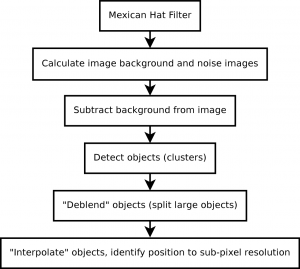
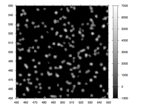
The bulk of the image analysis takes place in the \texttt{ImageData} object (stored in \texttt{ImageProcess.cpp/h}). Stages of the image analysis process are illustrated in figure~\ref{firecrest-imageanalysis-stages}. To illustrate the image analysis we’ll be looking at the processing of an example image. The original input image is shown in figure~\ref{firecrest-image-input}.
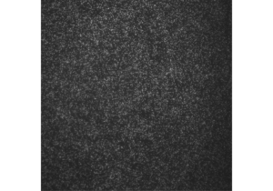
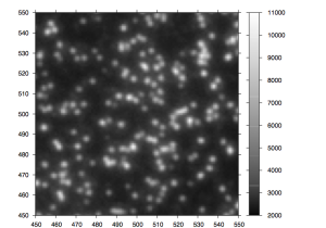
firecrest-image-input: An example input image and magnified selection.
The first stage of processing applies a Mexican Hat filter to the image. (NOTE: I guess attenuating low and high frequencies makes the image smoother and the edges stronger? Need to add more details.)


firecrest-image-post-mexicanhat: Image after Mexican hat filter.
\subsection{Noise estimation}
For noise estimation the image is broken in to a number of regions, for each region a single noise value is calculated. The image is broken in the smallest even number of regions greater than 125 pixels square. This value has been selected in order to provide enough samples to calculate noise (NOTE: from Klaus).
For each region an initial histogram with fine binning is created. The inital bin width is calculated as: $w = \frac{\sigma}{7\times50}$, where the standard deviation is calculated from the filtered image (in this region). That is, according the code comments, ten times finer than any interval, with an additional factor of 5 to account for the overestimation of noise dispersion in the original image. This value is rounded to the nearest power of 10. Seven has been selected heuristically based on the sample size. The minimum value stored in the histogram is $min = (\frac{\mu-2.5\times\sigma}{w}-0.5)\times w$, where the average is value calculated from the filter image in this region. The number of bins is calculated as $\frac{5\times\sigma}{w}$.
The histogram is then smoothed in three passes, or until smoothing no longer results in a tighter standard deviation. Smoothing is by “mean filtering”, this iterates over the histogram subtracting the value windowsize (of half the size of the s.d.) less than the current position and adding that windowsize greater.
A new histogram is then created based on these refined values. The binning width here is $\frac{\sigma}{7}$ (where $\sigma$ is the new sd). The minimum value to store in the histogram is calculated as $\mu-2\times\sigma-0.5w$. This histogram is clipped at such that only values $v+\sqrt{v} > m-\sqrt{m}\times e^{-0.5}$ (where $v$ is the value at in the histogram, and $m$ is the maximum value in the histogram).
If after clipping there are less than 5 bins, and additional bin is added to each slide of the histogram. If there are still less than 5 bins noise estimation fails. A gaussian is fitted to the resulting histogram. The average from the gaussian is used to populate the “background” image in this region, the standard deviation to population the “noise” image. Example background and noise images can been seen in figures~\ref{firecrest-image-background} and \ref{firecrest-image-noise}.

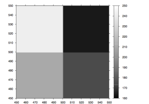
firecrest-image-noise: Noise image.

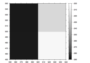
firecrest-image-background: Background image.
\subsection{Object Identification}
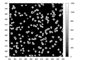
The background image (calculated during noise estimation) is subtracted from the filtered image (an example is shown in figure~\ref{firecrest-image-subtracted}). This image is then thresholded. Thresholding retains pixels whose value is greater than a “factor” multiplied by the associated pixel in the noise image. The factor currently used is 4. A thresholded image is shown in figure~\ref{firecrest-image-thresholded}.

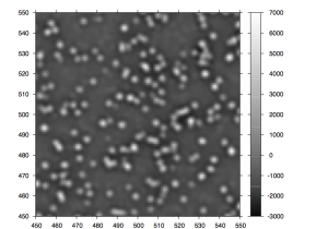
firecrest-image-subtracted: Image with background subtracted.
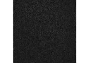
firecrest-image-thresholded: Image after thresholding.
After thresholding object detection takes place. The algorithm is reasonably straightforward. Every pixel in the image is itterated over when a pixel above the threshold in encountered a boundary is created. The boundary is created by walking all adjacent above threshold pixels clockwise. The area covered by this newly identified cluster is also calculated, and the pixels in this position on the original image unset (to avoid detecting this cluster again). During this process the maximum pixel intensity in this cluster is also found. It is the maximum pixel intensity that is passed to the base caller (rather than a function of all the pixels in this cluster). Initially identified clusters are shown in figure~\ref{firecrest-image-identifiedobjects}.

firecrest-image-identifiedobjects: Image after object identification, gray pixel indicate the maximum pixel identified in this object.
\subsubsection{Deblending}
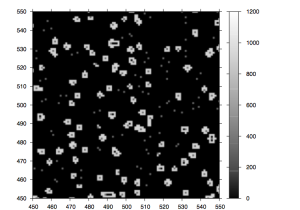
If an objects area is greater than $2f^2$ where $f$ is an input parameter and usually set at 2.7 the object is split. However if objects are too large (greater than $16f^2$) it is simply ignored (i.e. it is kept, there is a TODO suggesting it should be deleted in the source). I’m not sure how this is squared with the “many” clusters that are usually identified in blobs.

firecrest-image-deblended: Image after object deblending, gray pixels indicate the maximum pixel in this object. Split objects no longer have boundaries, and so only the maximum pixel is shown.
\subsubsection{Local Backgrond Compensation}
Once final objects have been identified local background can be compensated for. This is calculated in the function \texttt{get\_background\_dispersion} and subtracted from the cluster intensity in \texttt{integrate\_objects}. Local background compensation takes a 10×10 window around the pixel with maximum intensity in a cluster. All pixels that are not part of a cluster are extracted and sorted.
An iterative process then occurs such that (to quote the source): “The background is given by the median of the pixel distribution, and the noise is chosen such that 68\% of the pixels lie within a 2-sigma interval. The procedure is iterated and each time 3-sigma outliers are removed to avoid large contaminations by residual low-level signal.”
The background is therefore the median pixel, noise is calculated as: $\frac{c}{2}-0.34c – \frac{c}{2}+0.34c$ where $c$ is the number of pixels. This process occurs iteratively removing maximum pixels if they are greater than background = $3\times$noise. This iteration terminates if less than 2 pixels are removed or less than 20 pixels remain.
Bustard
Bustard is the Illumina basecaller, the base call is simply the maximum intensity after Crosstalk and Phasing corrections have been applied. Quality score calculation is more involved (NOTE: add more)
\section{Crosstalk matrix correction}
Crosstalk correct is perform as described for capillary sequence by Li and Speed~\cite{li98}.\section{Phasing correction}
Phasing is a term used to describe the signal contribution of bases from the previous and next cycles. Because the labelled base is not always successfully incorporated or two bases are incorporated instead of one this “signal leakage” sometimes occurs.
Phasing and prephasing are calculated as follows:
~
~
$phasing_b$ = average of previous cycle where $b$ is max – average of previous cycle where $b$ is NOT max
~
$prephasing_b$ = average of next cycle where $b$ is max – average of next cycle where $b$ is NOT max
~
~
Where $b$ is a given base. Phasing and prephasing are averaged over the run and used to derive a correction matrix. (NOTE: add detail and check)
\section{Basecalling}
(NOTE: add this)
Gerald
\section{Purity and Chastity}
Purity is defined as the ratio of the largest intensity to the sum of all intensities for this cycle/cluster. Chastity is a similar metric, and is defined as the ratio of the largest intensity to the sum of the largest and second largest intensities. As pointed out by Irina, the logic of this definition is somewhat faulty. If the second highest intensity is negative (as it can be due to background compensation) it will contribute to the sum incorrectly. To further complicate the situation Chastity is also sometimes used to mean a limit for purity (for example in PhasingEstimate.cpp). E.g. Chastity of 0.6 means to not accept purity above 0.6.
Purity and chastity are used as filters to identify mixed clusters, these are cluster which have grown from more than one molecule.
File Descriptions
\section{Initial run folder}
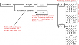
Before processing by the pipeline the run folder need only contain an Images directory and .params file. The params file should have the same name as the run folder.
The Images directory contains a subdirectory for each lane in the format \texttt{Lnnn} where \texttt{nnn} is the lane number. For example lane 1 would be \texttt{L001}. The lane directory contains a subdirectory for each cycle, the Solexa run folder documentation states that this is in \texttt{C
\subsection{.params file}
The \texttt{.params} file is in the root of the run folder and must have the same name as the run folder. It’s an xml format file, and it’s general format can be seen in the following example:
\VerbatimInput{examples/myfake.params}
Figure~\ref{runfolder-initial} gives an overview of the initial run folder structure.
runfolder_initial: Initial run folder structure, folders are represented by boxes, unboxed items are files.
\section{Pipefile files, before run}
To run the pipeline, you first tell it to create a set of makefiles in the run folder. For our \texttt{myfakerun} folder we might execute the following command to do this:
\begin{center}
\texttt{./GAPipeline-0.3.0b3/Goat/goat\_pipeline.py –cycles=1-36 myfakerun –make}
\end{center}
This creates a \texttt{Data} directory and populates it with files, note you need to tell the pipeline how many cycles ran. The \texttt{Data} directory contains a directory with a name similar to the following:
\begin{center}
\texttt{C1-36\_Firecrest1.9.2\_07-01-2008\_username}
\end{center}
This is named after the cycle numbers, Firecrest version number (?), date and username of the user who ran the software. A breakdown of this directory structure with additional directories highlighted is shown in~\ref{runfolder-makefilescreated}.
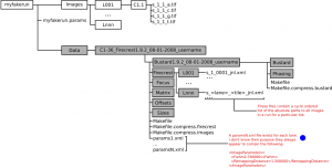
runfolder-makefilescreated: Run folder, after the pipeline has created it’s initial Makefiles. New folders are highlighted in grey. Blue dots highlight files of unknown function.
\section{Firecrest}
After firecrest (the Solexa image analysis tool) has run a huge number of files are created, these are described in figure~\ref{runfolder-postfirecrest}. From our perspective the most useful of these files are the \texttt{s\_
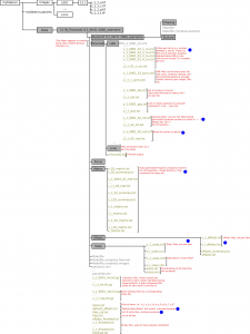
runfolder-postfirecrest: Run folder, after firecrest run. New files are highlighted in Olive. Blue dots indicate files of unknown function.
\section{Bustard}
Bustard, the Solexa base caller, also creates a large number of files, from a user perspective the \texttt{s\_
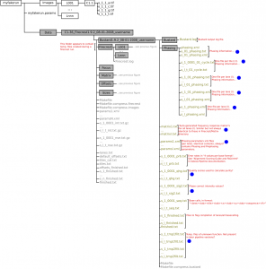
runfolder-postbustard: Run folder, after Bustard run. New files are highlighted in Olive. Blue dots indicate files of unknown/unclear function.
\section{Gerald}
In order to run Gerald, you need a Gerald configuration file. The format is quite straight forward and is described in \texttt{GERALD User Guide and FAQ.html} in the Solexa pipeline documentation. An example, simple configuration might be:
\VerbatimInput{examples/gerald.config}
Once you have a configuration file, you can ask Gerald to create a set of Makefiles with the following command (one line):
~
\scriptsize
\texttt{./GAPipeline-0.3.0b3/Gerald/GERALD.pl ./myfake/gerald.config}
\texttt{–EXPT\_DIR}
\texttt{ ./myfake/Data/C1-36\_Firecrest1.9.2\_08-01-2008\_username/Bustard1.9.2\_08-01-2008\_username –FORCE}
\normalsize
~
This creates a directory with the name \texttt{GERALD\_08-01-2008\_username} (where 8-01-2008 is the current date), under the \texttt{Bustard1.9.2\_08-01-2008\_username} directory. This contains a copy of the configuration file originally provided (\texttt{config.txt}) and version of this file converted in to xml format (\texttt{config.xml}) and a makefile. To run Gerald, simply run make. The \texttt{htm} files in this directory contain run reports, details of error rates, signal intensities etc. The most useful files in this directory are the \texttt{s\_
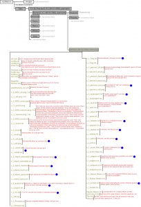
runfolder-postgerald: Run folder, after Gerald run. New files are highlighted in Olive. Blue dots indicate files of unknown/unclear function.
